
Python:PyTorch 推理和验证 (七十九)
推理与验证
在训练神经网络之后,你现在可以使用它来进行预测。这种步骤通常被称作推理,这是一个借自统计学的术语。然而,神经网络在面对训练数据时往往表现得太过优异,因而无法泛化未见过的数据。这种现象被称作过拟合,它损害了推理性能。为了在训练时检测过拟合,我们测量并不在名为验证集的训练集中数据的性能。在训练时,我们一边监控验证性能,一边进行正则化,如 Dropout,以此来避免过拟合。在这个 notebook 中,我将向你展示如何在 PyTorch 中做到这一点。
首先,我会实现我自己的前馈神经网络,这个网络基于第四部分的练习中的 Fashion-MNIST 数据集构建。它是第四部分练习的解决方案,也是如何进行 Dropout 和验证的例子。
向往常一样,我们先通过 torchvision 来加载数据集。你将会在下一部分更深入地学习有关 torchvision 和加载数据的知识。
%matplotlib inline
%config InlineBackend.figure_format = 'retina'

import matplotlib.pyplot as plt
import numpy as np
import time

import torch
from torch import nn
from torch import optim
import torch.nn.functional as F
from torch.autograd import Variable
from torchvision import datasets, transforms

import helper
# Define a transform to normalize the data
transform = transforms.Compose([transforms.ToTensor(),
transforms.Normalize((0.5, 0.5, 0.5), (0.5, 0.5, 0.5))])
# Download and load the training data
trainset = datasets.FashionMNIST('F_MNIST_data/', download=True, train=True, transform=transform)
trainloader = torch.utils.data.DataLoader(trainset, batch_size=64, shuffle=True)
# Download and load the test data
testset = datasets.FashionMNIST('F_MNIST_data/', download=True, train=False, transform=transform)
testloader = torch.utils.data.DataLoader(testset, batch_size=64, shuffle=True)构建网络
跟 MNIST 数据集一样,Fashion-MNIST 数据集中每张图片的像素为 28x28,共 784 个数据点和 10 个类。我使用了 nn.ModuleList 来加入任意数量的隐藏层。这个模型中的 hidden_layers 参数为隐藏层大小的列表(以整数表示)。使用 nn.ModuleList 来寄存每一个隐藏模块,这样你可以在之后使用模块方法。
我还使用了 forward 方法来返回输出的 log-softmax。由于 softmax 是类的概率分布,因此 log-softmax 是一种对数概率,它有许多优点。使用这种对数概率,计算往往会更加迅速和准确。为了在之后获得类的概率,我将需要获得输出的指数(torch.exp)。
我们可以使用 nn.Dropout 来在我们的网络中加入 Dropout。这与 nn.Linear 等其他模块的作用相似。它还将 Dropout 概率作为一种输入传递到网络中。
class Network(nn.Module):
    def __init__(self, input_size, output_size, hidden_layers, drop_p=0.5):
        ''' Builds a feedforward network with arbitrary hidden layers.

            Arguments
            ---------
            input_size: integer, size of the input
            output_size: integer, size of the output layer
            hidden_layers: list of integers, the sizes of the hidden layers
            drop_p: float between 0 and 1, dropout probability
        '''
        super().__init__()
        # Add the first layer, input to a hidden layer
        self.hidden_layers = nn.ModuleList([nn.Linear(input_size, hidden_layers[0])])

        # Add a variable number of more hidden layers
        layer_sizes = zip(hidden_layers[:-1], hidden_layers[1:])
        self.hidden_layers.extend([nn.Linear(h1, h2) for h1, h2 in layer_sizes])

        self.output = nn.Linear(hidden_layers[-1], output_size)

        self.dropout = nn.Dropout(p=drop_p)

    def forward(self, x):
        ''' Forward pass through the network, returns the output logits '''

        for each in self.hidden_layers:
            x = F.relu(each(x))
            x = self.dropout(x)
        x = self.output(x)

        return F.log_softmax(x, dim=1)
训练网络
由于该模型的前向方法返回 log-softmax,因此我使用了负对数损失 作为标准。我还选用了Adam 优化器。这是一种随机梯度下降的变体,包含了动量,并且训练速度往往比基本的 SGD 要快。
我还加入了一个代码块来测量验证损失和精确度。由于我在这个神经网络中使用了 Dropout,在推理时我需要将其关闭,否则这个网络将会由于许多连接的关闭而表现糟糕。在 PyTorch 中,你可以使用 model.train() 和 model.eval() 来将模型调整为“训练模式”或是“评估模式”。在训练模式中,Dropout 为开启状态,而在评估模式中,Dropout 为关闭状态。这还会影响到其他模块,包括那些应该在训练时开启、在推理时关闭的模块。
这段验证代码由一个通过验证集(并分裂成几个批次)的前向传播组成。我根据 log-softmax 输出来计算验证集的损失以及预测精确度。
# Create the network, define the criterion and optimizer
model = Network(784, 10, [500], drop_p=0.5)
criterion = nn.NLLLoss()
optimizer = optim.Adam(model.parameters(), lr=0.001)
epochs = 2
steps = 0
running_loss = 0
print_every = 40
for e in range(epochs):
# Model in training mode, dropout is on
model.train()
for images, labels in iter(trainloader):
steps += 1
# Flatten images into a 784 long vector
images.resize_(images.size()[0], 784)
# Wrap images and labels in Variables so we can calculate gradients
inputs = Variable(images)
targets = Variable(labels)
optimizer.zero_grad()
output = model.forward(inputs)
loss = criterion(output, targets)
loss.backward()
optimizer.step()
running_loss += loss.data[0]
if steps % print_every == 0:
# Model in inference mode, dropout is off
model.eval()
accuracy = 0
test_loss = 0
for ii, (images, labels) in enumerate(testloader):
images = images.resize_(images.size()[0], 784)
# Set volatile to True so we don't save the history
inputs = Variable(images, volatile=True)
labels = Variable(labels, volatile=True)
output = model.forward(inputs)
test_loss += criterion(output, labels).data[0]
## Calculating the accuracy
# Model's output is log-softmax, take exponential to get the probabilities
ps = torch.exp(output).data
# Class with highest probability is our predicted class, compare with true label
equality = (labels.data == ps.max(1)[1])
# Accuracy is number of correct predictions divided by all predictions, just take the mean
accuracy += equality.type_as(torch.FloatTensor()).mean()
print("Epoch: {}/{}.. ".format(e+1, epochs),
"Training Loss: {:.3f}.. ".format(running_loss/print_every),
"Test Loss: {:.3f}.. ".format(test_loss/len(testloader)),
"Test Accuracy: {:.3f}".format(accuracy/len(testloader)))
running_loss = 0
# Make sure dropout is on for training
model.train()/opt/conda/lib/python3.6/site-packages/ipykernel_launcher.py:23: UserWarning: invalid index of a 0-dim tensor. This will be an error in PyTorch 0.5. Use tensor.item() to convert a 0-dim tensor to a Python number
/opt/conda/lib/python3.6/site-packages/ipykernel_launcher.py:35: UserWarning: volatile was removed and now has no effect. Use `with torch.no_grad():` instead.
/opt/conda/lib/python3.6/site-packages/ipykernel_launcher.py:36: UserWarning: volatile was removed and now has no effect. Use `with torch.no_grad():` instead.
/opt/conda/lib/python3.6/site-packages/ipykernel_launcher.py:39: UserWarning: invalid index of a 0-dim tensor. This will be an error in PyTorch 0.5. Use tensor.item() to convert a 0-dim tensor to a Python number
Epoch: 1/2.. Training Loss: 1.049.. Test Loss: 0.705.. Test Accuracy: 0.732
Epoch: 1/2.. Training Loss: 0.730.. Test Loss: 0.637.. Test Accuracy: 0.766
Epoch: 1/2.. Training Loss: 0.641.. Test Loss: 0.583.. Test Accuracy: 0.784
Epoch: 1/2.. Training Loss: 0.602.. Test Loss: 0.566.. Test Accuracy: 0.786
Epoch: 1/2.. Training Loss: 0.564.. Test Loss: 0.543.. Test Accuracy: 0.798
Epoch: 1/2.. Training Loss: 0.587.. Test Loss: 0.513.. Test Accuracy: 0.815
Epoch: 1/2.. Training Loss: 0.582.. Test Loss: 0.531.. Test Accuracy: 0.805
Epoch: 1/2.. Training Loss: 0.563.. Test Loss: 0.525.. Test Accuracy: 0.803
Epoch: 1/2.. Training Loss: 0.544.. Test Loss: 0.484.. Test Accuracy: 0.824
Epoch: 1/2.. Training Loss: 0.518.. Test Loss: 0.486.. Test Accuracy: 0.824
Epoch: 1/2.. Training Loss: 0.510.. Test Loss: 0.479.. Test Accuracy: 0.822
Epoch: 1/2.. Training Loss: 0.516.. Test Loss: 0.485.. Test Accuracy: 0.817
Epoch: 1/2.. Training Loss: 0.486.. Test Loss: 0.484.. Test Accuracy: 0.824
Epoch: 1/2.. Training Loss: 0.515.. Test Loss: 0.465.. Test Accuracy: 0.827
Epoch: 1/2.. Training Loss: 0.509.. Test Loss: 0.479.. Test Accuracy: 0.826
Epoch: 1/2.. Training Loss: 0.471.. Test Loss: 0.471.. Test Accuracy: 0.829
Epoch: 1/2.. Training Loss: 0.487.. Test Loss: 0.456.. Test Accuracy: 0.833
Epoch: 1/2.. Training Loss: 0.476.. Test Loss: 0.462.. Test Accuracy: 0.833
Epoch: 1/2.. Training Loss: 0.482.. Test Loss: 0.455.. Test Accuracy: 0.833
Epoch: 1/2.. Training Loss: 0.505.. Test Loss: 0.443.. Test Accuracy: 0.837
Epoch: 1/2.. Training Loss: 0.482.. Test Loss: 0.447.. Test Accuracy: 0.836
Epoch: 1/2.. Training Loss: 0.487.. Test Loss: 0.439.. Test Accuracy: 0.840
Epoch: 1/2.. Training Loss: 0.470.. Test Loss: 0.446.. Test Accuracy: 0.837
Epoch: 2/2.. Training Loss: 0.504.. Test Loss: 0.432.. Test Accuracy: 0.845
Epoch: 2/2.. Training Loss: 0.468.. Test Loss: 0.451.. Test Accuracy: 0.837
Epoch: 2/2.. Training Loss: 0.449.. Test Loss: 0.464.. Test Accuracy: 0.825
Epoch: 2/2.. Training Loss: 0.457.. Test Loss: 0.434.. Test Accuracy: 0.841
Epoch: 2/2.. Training Loss: 0.463.. Test Loss: 0.445.. Test Accuracy: 0.838
Epoch: 2/2.. Training Loss: 0.437.. Test Loss: 0.436.. Test Accuracy: 0.844
Epoch: 2/2.. Training Loss: 0.463.. Test Loss: 0.447.. Test Accuracy: 0.842
Epoch: 2/2.. Training Loss: 0.487.. Test Loss: 0.436.. Test Accuracy: 0.842
Epoch: 2/2.. Training Loss: 0.444.. Test Loss: 0.442.. Test Accuracy: 0.839
Epoch: 2/2.. Training Loss: 0.459.. Test Loss: 0.461.. Test Accuracy: 0.830
Epoch: 2/2.. Training Loss: 0.463.. Test Loss: 0.430.. Test Accuracy: 0.841
Epoch: 2/2.. Training Loss: 0.492.. Test Loss: 0.435.. Test Accuracy: 0.841
Epoch: 2/2.. Training Loss: 0.451.. Test Loss: 0.416.. Test Accuracy: 0.850
Epoch: 2/2.. Training Loss: 0.453.. Test Loss: 0.428.. Test Accuracy: 0.846
Epoch: 2/2.. Training Loss: 0.465.. Test Loss: 0.471.. Test Accuracy: 0.826
Epoch: 2/2.. Training Loss: 0.476.. Test Loss: 0.418.. Test Accuracy: 0.846
Epoch: 2/2.. Training Loss: 0.457.. Test Loss: 0.417.. Test Accuracy: 0.844
Epoch: 2/2.. Training Loss: 0.427.. Test Loss: 0.422.. Test Accuracy: 0.847
Epoch: 2/2.. Training Loss: 0.425.. Test Loss: 0.436.. Test Accuracy: 0.844
Epoch: 2/2.. Training Loss: 0.449.. Test Loss: 0.415.. Test Accuracy: 0.852
Epoch: 2/2.. Training Loss: 0.428.. Test Loss: 0.411.. Test Accuracy: 0.850
Epoch: 2/2.. Training Loss: 0.449.. Test Loss: 0.419.. Test Accuracy: 0.848
Epoch: 2/2.. Training Loss: 0.424.. Test Loss: 0.411.. Test Accuracy: 0.850推理
模型已经训练好了,我们现在可以使用它来进行推理。之前已经进行过这一步骤,但现在我们需要使用 model.eval() 来将模型设置为推理模式。
# Test out your network!

model.eval()

dataiter = iter(testloader)
images, labels = dataiter.next()
img = images[0]
# Convert 2D image to 1D vector
img = img.resize_(1, 784)

# Calculate the class probabilities (softmax) for img
output = model.forward(Variable(img, volatile=True))
ps = torch.exp(output)

# Plot the image and probabilities
helper.view_classify(img.resize_(1, 28, 28), ps)
/opt/conda/lib/python3.6/site-packages/ipykernel_launcher.py:12: UserWarning: volatile was removed and now has no effect. Use `with torch.no_grad():` instead.
if sys.path[0] == '':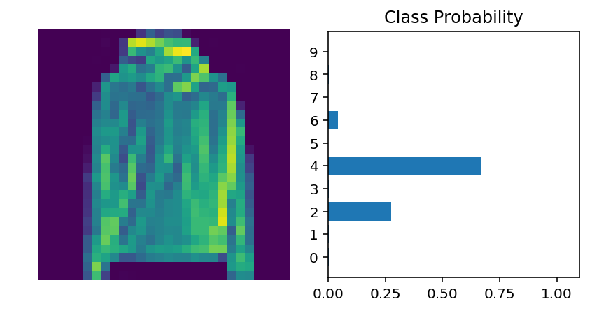
下一步!
在下一部分,我将为你展示如何保存训练好的模型。一般来说,你不会希望在每次使用模型时都要重新训练,而是希望在训练好模型之后将其保存,以便下次训练或推理时使用。
为者常成,行者常至
自由转载-非商用-非衍生-保持署名(创意共享3.0许可证)


