
AI 量化交易-基础成对交易算法实现 (二)
【实战】基础成对交易算法实现
数据获得
想要做量化,首先你得有数据。股市的交易数据的来源可以有很多地方,比如直接对接交易所,比如从万徳,彭博社,路透社等数据第三方。当然,以上大部分都是收费的,企业用户用起来无压力,个人用户就有点吃力了。所以我这里还推荐一些免费的交易数据网站,大家可以玩一玩:
http://www.financialcontent.com/
https://www.quandl.com/ (教育目的免费)
他们都提供很直观便捷的API,大家注册一下就可以了,然后就可以下载或者导入自己需要的数据资源。
选取目标股票
假设,按照我们前面讲的理论,我们找一些相同行业内的企业,来首先保证他们之间有足够强的内在经济联系
我来举几个大家熟悉的美股饮料公司的股票:

import pandas as pd从各种可行的数据源下载或者导入这些股票的历史交易记录,并读入
data_PEP = pd.read_csv('./data/daily_PEP.csv', index_col=[0],usecols=['timestamp','close'])
data_PEP.columns = ["PEP"]
data_KO = pd.read_csv('./data/daily_KO.csv', index_col=[0],usecols=['timestamp','close'])
data_KO.columns = ["KO"]
data_KDP = pd.read_csv('./data/daily_KDP.csv', index_col=[0],usecols=['timestamp','close'])
data_KDP.columns = ["KDP"]
data_MNST = pd.read_csv('./data/daily_MNST.csv', index_col=[0],usecols=['timestamp','close'])
data_MNST.columns = ["MNST"]
我们暂时不需要所有的信息,只需要每天的closing price,所以,我们精简一下数据
print(data_PEP) PEP
timestamp
2018-12-13 118.35
2018-12-12 117.00
2018-12-11 117.29
2018-12-10 116.19
2018-12-07 115.82
2018-12-06 116.84
2018-12-04 117.80
2018-12-03 118.98
2018-11-30 121.94
2018-11-29 118.27
2018-11-28 118.50
2018-11-27 116.44
2018-11-26 115.86
2018-11-23 115.41
2018-11-21 115.28
2018-11-20 116.00
... ...
1998-01-27 36.06
1998-01-05 36.50
1998-01-02 36.00
[5272 rows x 1 columns]把所有的数据都塞在一起
data = pd.concat([data_PEP,data_KO,data_KDP, data_MNST,],axis=1,)
print(data)
PEP KO KDP MNST
1998-01-02 36.00 66.94 NaN 1.810
1998-01-05 36.50 66.44 NaN 1.781
1998-01-06 35.19 66.13 NaN 1.750
1998-01-07 35.88 66.19 NaN 1.719
1998-01-08 35.88 66.63 NaN 1.813
1998-01-09 34.75 64.13 NaN 1.625
1998-01-12 35.38 66.06 NaN 1.500
1998-01-13 36.50 65.38 NaN 1.500
1998-01-14 36.69 64.63 NaN 1.469
1998-01-15 35.94 63.75 NaN 1.625
1998-01-16 36.69 65.00 NaN 1.688
1998-01-20 37.63 65.94 NaN 1.656
1998-01-21 37.00 65.50 NaN 1.750
1998-01-22 36.88 65.44 NaN 1.563
1998-01-23 36.31 63.81 NaN 1.563
1998-01-26 36.44 63.06 NaN 1.719
... ... ... ... ...
2018-10-31 112.38 47.88 26.00 52.850
2018-11-01 111.51 47.74 26.52 54.450
2018-12-11 117.29 49.54 26.29 57.580
2018-12-12 117.00 49.22 26.12 57.440
2018-12-13 118.35 49.47 26.15 53.430
[5272 rows x 4 columns]
/opt/conda/lib/python3.5/site-packages/ipykernel_launcher.py:1: FutureWarning: Sorting because non-concatenation axis is not aligned. A future version
of pandas will change to not sort by default.
To accept the future behavior, pass 'sort=False'.
To retain the current behavior and silence the warning, pass 'sort=True'.
"""Entry point for launching an IPython kernel.只为案例:我们这里挑个时间段 2015-05-01 ~ 2016-05-01
data = data['2016-03-01':'2016-10-01']除此之外,我们还要把数据中的Nan给解决好。比如,如果当日的close是Nan,说明要么数据遗漏,要么当日没有开,那么我们沿用前一天的价格
data.fillna(method='ffill')| PEP | KO | KDP | MNST | |
|---|---|---|---|---|
| 2016-03-01 | 99.09 | 43.69 | 92.71 | 129.73 |
| 2016-03-02 | 98.33 | 43.77 | 91.98 | 127.75 |
| 2016-03-03 | 99.16 | 43.96 | 91.95 | 128.47 |
| 2016-03-04 | 100.00 | 44.11 | 91.78 | 128.89 |
| 2016-03-07 | 99.25 | 44.01 | 90.21 | 127.99 |
| 2016-03-08 | 99.74 | 44.32 | 90.75 | 129.33 |
| 2016-03-09 | 100.20 | 44.81 | 92.02 | 130.07 |
| 2016-03-10 | 100.78 | 45.23 | 92.12 | 131.65 |
| 2016-03-11 | 101.31 | 45.20 | 91.04 | 133.86 |
| 2016-03-14 | 100.65 | 45.29 | 90.75 | 131.96 |
| 2016-03-18 | 101.29 | 45.60 | 90.35 | 136.53 |
| 2016-03-21 | 101.54 | 45.67 | 90.24 | 134.52 |
| 2016-03-22 | 100.77 | 45.50 | 89.37 | 134.60 |
| 2016-03-23 | 100.81 | 45.46 | 89.96 | 132.83 |
| 2016-03-24 | 100.68 | 45.58 | 88.23 | 131.25 |
| 2016-09-07 | 107.21 | 43.64 | 93.55 | 152.17 |
| 2016-09-08 | 106.88 | 43.63 | 92.99 | 152.12 |
| 2016-09-09 | 104.05 | 42.27 | 89.84 | 147.55 |
| 2016-09-12 | 106.02 | 43.19 | 91.26 | 148.30 |
150 rows × 4 columns
# n = data.shape
# print(n)
# (150, 4)

# type(data)
# pandas.core.frame.DataFrame

# row_n = 4
# score_matrix = np.zeros((row_n, row_n))
# score_matrix[:2]

# pvalue_matrix = np.ones((row_n, row_n))
# pvalue_matrix

keys = data.keys()
print(keys)
Index(['PEP', 'KO', 'KDP', 'MNST'], dtype='object')寻找Cointegration
我们这一个步骤来做这件事:
对于所有的目标池内的股票,我们计算他们是否各自Coint:
# 两两配对,算一下Coint
def find_cointegrated_pairs(data):
    n = data.shape[1]
    score_matrix = np.zeros((n, n))
    pvalue_matrix = np.ones((n, n))
    keys = data.keys()
    pairs = []
    for i in range(n):
        for j in range(i+1, n):
            S1 = data[keys[i]]
            S2 = data[keys[j]]
            result = coint(S1, S2)
            score = result[0]
            pvalue = result[1]
            score_matrix[i, j] = score
            pvalue_matrix[i, j] = pvalue
            if pvalue < 0.05:
                pairs.append((keys[i], keys[j]))
    return score_matrix, pvalue_matrix, pairs
我们把算出来的数值都画出来,可以直观的看到哪一对最好:
import numpy as np
from statsmodels.tsa.stattools import coint
%matplotlib inline

scores, pvalues, pairs = find_cointegrated_pairs(data)
import seaborn

# 直观点把这个图画出来
seaborn.heatmap(pvalues, xticklabels=['PEP','KO','KDP','MNST'], yticklabels=['PEP','KO','KDP','MNST'], cmap='RdYlGn_r'
                , mask = (pvalues >= 0.05)
                )
/opt/conda/lib/python3.5/site-packages/statsmodels/compat/pandas.py:56: FutureWarning: The pandas.core.datetools module is deprecated and will be removed in a future version. Please use the pandas.tseries module instead.
from pandas.core import datetools
<matplotlib.axes._subplots.AxesSubplot at 0x7f70b5a34470>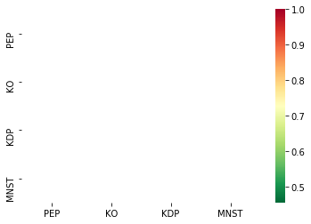
由图可见,我们可以挑 ['KDP', 'MNST'] 这一对,作为我们重点考察目标:
S1 = data['KDP']
S2 = data['MNST']
我们来看看此刻的P-value是多少
score, pvalue, _ = coint(S1, S2)
pvalue0.4548934445039827计算Spread
按照之前讲的套路,计算S1和S2的OLS,得到我们的spread,并画出图像
import statsmodels
import statsmodels.api as sm
import matplotlib.pyplot as plt

print("S1\n",S1.head(5))
S1 = sm.add_constant(S1)
print("S1-constant\n", S1.head(5))

# OLS 最小二乘法
results = sm.OLS(S2, S1).fit()
S1 = S1['KDP']
print("results:\n", results.params);

# 打印出一个模型的诊断细节
print("results.summary:\n", results.summary());

b = results.params['KDP']

spread = S2 - b * S1
spread.plot()
plt.axhline(spread.mean(), color='black')
plt.legend(['Spread']);
S1
2018-03-01 116.44
2018-03-02 116.24
2018-03-05 115.91
2018-03-06 116.12
2018-03-07 116.30
Name: KDP, dtype: float64
S1-constant
const KDP
2018-03-01 1.0 116.44
2018-03-02 1.0 116.24
2018-03-05 1.0 115.91
2018-03-06 1.0 116.12
2018-03-07 1.0 116.30
results:
const 61.59733
KDP -0.05579
dtype: float64
results.summary:
OLS Regression Results
==============================================================================
Dep. Variable: MNST R-squared: 0.533
Model: OLS Adj. R-squared: 0.530
Method: Least Squares F-statistic: 167.7
Date: Sun, 06 Oct 2019 Prob (F-statistic): 4.51e-26
Time: 08:17:25 Log-Likelihood: -345.15
No. Observations: 149 AIC: 694.3
Df Residuals: 147 BIC: 700.3
Df Model: 1
Covariance Type: nonrobust
==============================================================================
coef std err t P>|t| [0.025 0.975]
------------------------------------------------------------------------------
const 61.5973 0.406 151.771 0.000 60.795 62.399
KDP -0.0558 0.004 -12.950 0.000 -0.064 -0.047
==============================================================================
Omnibus: 20.992 Durbin-Watson: 0.141
Prob(Omnibus): 0.000 Jarque-Bera (JB): 25.176
Skew: -0.979 Prob(JB): 3.41e-06
Kurtosis: 3.469 Cond. No. 189.
==============================================================================
Warnings:
[1] Standard Errors assume that the covariance matrix of the errors is correctly specified.
按照标准measurement,算个Standard Score,这样我们可以清楚看到基准线(=0),也可以很轻松的画出两条边际线
def zscore(series):
    return (series - series.mean()) / np.std(series)
此刻,我们就可以按照+1.0和-1.0的,画出两条指导线了
zscore(spread).plot()
plt.axhline(zscore(spread).mean(), color='black')
plt.axhline(1.0, color='red', linestyle='--')
plt.axhline(-1.0, color='green', linestyle='--')
plt.legend(['Spread z-score', 'Mean', '+1', '-1']);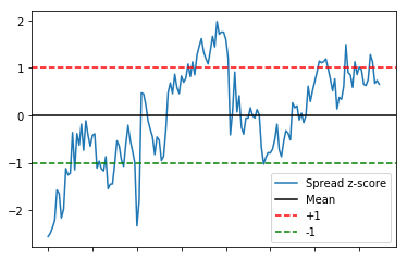
我们的策略行动很简单粗暴:
- 当波动低于-1.0的线,Long the spread
- 当波动高于1.0的线,Short the spread
- 当波动接近于0,退出Hedged Position
【实战】优化版的成对交易模型
Moving Average
既然是滚动平均值,那我们就需要一个滚动的OLS来计算每一次:
from pyfinance.ols import PandasRollingOLS
rolling_beta = PandasRollingOLS(y=S1, x=S2, window=30)
print(rolling_beta.beta.head())
feature1
2016-04-12 -0.119287
2016-04-13 -0.063562
2016-04-14 0.018802
2016-04-15 0.094118
2016-04-18 0.151175然后,我们用这个滚动的OLS,去计算滚动的平均值:
spread = S2 - rolling_beta.beta['feature1'] * S1
spread.name = 'spread'

# 画出每一天的MAVG
spread_mavg1 = spread.rolling(window=1).mean()
spread_mavg1.name = 'spread 1d mavg'

# 画出每30天的MAVG
spread_mavg30 = spread.rolling(window=30).mean()
spread_mavg30.name = 'spread 30d mavg'

plt.plot(spread_mavg1.index, spread_mavg1.values)
plt.plot(spread_mavg30.index, spread_mavg30.values)

plt.legend(['1 Day Spread MAVG', '30 Day Spread MAVG'])

plt.ylabel('Spread');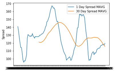
大家看到,楼上的滚动平均值更加的平滑,并且我们更准确清晰地知道什么时候我们要采取什么策略。
相比于单独的一个全局平均值,滚动平均值会随着市场的变化而变化,更加符合我们曲线的走势。
既然我们有了1天和30天的spread,我们就可以把这两个值当作我们的x和y,并用他们计算出一个统一的standard score,
面对这个zscore,我们可以更加直观的看出来我们的股票价格在什么时间点处于“极端值”:
# Take a rolling 30 day standard deviation
std_30 = spread.rolling(window=30).std()
std_30.name = 'std 30d'

# Compute the z score for each day
zscore_30_1 = (spread_mavg1 - spread_mavg30)/std_30
zscore_30_1.name = 'z-score'
zscore_30_1.plot()
plt.axhline(0, color='black')
plt.axhline(1.0, color='red', linestyle='--')
plt.axhline(-1.0, color='green', linestyle='--');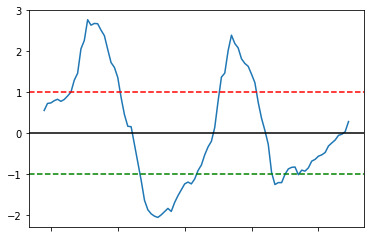
好,为了更加清晰地给大家看看我们这个走势变化与真实股票的关系,
我们可以把三个线 都画在同一个坐标系内:
# Plot the prices scaled down along with the negative z-score
# just divide the stock prices by 10 to make viewing it on the plot easier
plt.plot(S1.index, S1.values/10)
plt.plot(S2.index, S2.values/10)
plt.plot(zscore_30_1.index, zscore_30_1.values)
plt.legend(['S1 Price / 10', 'S2 Price / 10', 'Price Spread Rolling z-Score']);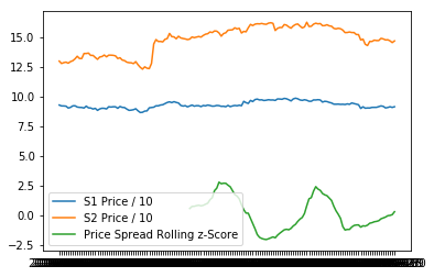
Out of Sample
如果我们的目标数据在我们考察的时间段范围以外怎么办?这样我们就需要再做一次Coint测试
比如,我们拿出一个S1与S2在新的时间段中的数据比较:
data_KDP = pd.read_csv('./data/daily_KDP.csv', index_col=[0],usecols=['timestamp','close'])
data_KDP.columns = ["KDP"]
data_MNST = pd.read_csv('./data/daily_MNST.csv', index_col=[0],usecols=['timestamp','close'])
data_MNST.columns = ["MNST"]
data = pd.concat([data_KDP, data_MNST,],axis=1,)
data = data['2018-03-01':'2018-10-01']
data.fillna(method='ffill')
/opt/conda/lib/python3.5/site-packages/ipykernel_launcher.py:5: FutureWarning: Sorting because non-concatenation axis is not aligned. A future version
of pandas will change to not sort by default.
To accept the future behavior, pass 'sort=False'.
To retain the current behavior and silence the warning, pass 'sort=True'.
"""| KDP | MNST | |
|---|---|---|
| 2018-03-01 | 116.44 | 54.22 |
| 2018-03-02 | 116.24 | 54.16 |
| 2018-03-05 | 115.91 | 55.74 |
| 2018-03-06 | 116.12 | 55.67 |
| 2018-03-07 | 116.30 | 55.55 |
| ... | ... | ... |
| 2018-10-01 | 23.10 | 57.36 |
149 rows × 2 columns
S1 = data['KDP']
S2 = data['MNST']
score, pvalue, _ = coint(S1, S2)
print(pvalue)0.5241888917528962看,这个值明显大于了我们的threshold 0.05,所以我们就不可以再用他们两对来进行成对交易。
所以这个时候,我们就该退出我们的交易策略,并寻找新的可能性机会。
为者常成,行者常至
自由转载-非商用-非衍生-保持署名(创意共享3.0许可证)


