
AI 量化交易-基于单因子回测的因子有效性验证 (三)
基于单因子回测的因子有效性验证
import pandas as pd
import numpy as np
import math
import matplotlib.pyplot as plt
f1=pd.read_pickle("./data/f1")
f2=pd.read_pickle("./data/f2")
f3=pd.read_pickle("./data/f3")
f4=pd.read_pickle("./data/f4")
f5=pd.read_pickle("./data/f5")
f6=pd.read_pickle("./data/f6")
f7=pd.read_pickle("./data/f7")
f8=pd.read_pickle("./data/f8")
f9=pd.read_pickle("./data/f9")
zz500_close=pd.read_pickle("./data/500_close")
stock_close=pd.read_pickle("./data/stock_close")

# print(type(f1))  # DataFrame 类型
# print(f1.head(5))
# print(f2.head(5))

#print(zz500_close.head(5))
#print(stock_close.head(5))

factors=[]     # dataframe转为list数据类型
factors.append(f1)
factors.append(f2)
factors.append(f3)
factors.append(f4)
factors.append(f5)
factors.append(f6)
factors.append(f7)
factors.append(f8)
factors.append(f9)
# 打印数据
print(factors[0])
000006.SZ 000021.SZ 000028.SZ 000030.SZ 000031.SZ 000042.SZ \
2014-01-02 0.223619 0.431191 0.462519 0.480099 0.194684 0.276364
2014-01-03 0.230574 0.432788 0.438171 0.451811 0.184918 0.273993
2014-01-06 0.236310 0.482473 0.453755 0.428896 0.178864 0.278375
2014-01-07 0.242048 0.543898 0.470441 0.403748 0.179281 0.286026
2014-01-08 0.234513 0.566307 0.496687 0.358242 0.179065 0.271463
2014-01-09 0.246907 0.553260 0.495461 0.343971 0.178381 0.222859
2014-01-10 0.182756 0.541446 0.505784 0.315592 0.159304 0.190332
2014-01-13 0.156648 0.549546 0.495279 0.232491 0.141089 0.147643
2014-01-14 0.158903 0.551803 0.493612 0.220879 0.150756 0.142306
2014-01-15 0.154856 0.584402 0.496859 0.179185 0.148817 0.136219
2014-01-16 0.156038 0.507767 NaN 0.133522 0.149453 0.136637
2014-01-17 0.165703 0.498301 0.503578 0.158781 0.153497 0.178689
2014-01-20 0.179021 0.514894 0.442791 0.183130 0.157330 0.174789
2014-01-21 0.199249 0.545728 0.380227 0.225633 0.152853 0.152064
... ... ... ... ... ... ...
603077.SH 603366.SH 603766.SH
2014-01-02 NaN 0.307698 0.538916
2014-01-03 NaN 0.281336 0.513972
2014-01-06 NaN 0.310322 0.505673
2014-01-07 NaN 0.347464 0.531060
2014-01-08 NaN 0.388603 0.531166
2014-01-09 0.524233 0.396467 0.472439
2014-01-10 0.522978 0.399650 0.437208
2014-01-13 0.514245 0.395812 0.437932
2014-01-14 0.511321 0.396745 0.435420
2014-01-15 0.496796 0.409637 0.431013
2014-01-16 0.472812 0.398941 0.451205
2014-01-17 0.402493 0.398496 0.464105
2014-01-20 0.369810 0.392815 0.476474
2014-01-21 0.371354 0.369807 0.525631
2014-01-22 0.351603 0.355997 0.580023
2014-01-23 0.341845 0.327986 0.581361
2014-01-24 0.348250 0.330981 0.645134
2014-01-27 0.380139 0.326159 0.626267
2014-01-28 0.351959 0.322979 0.602506
2014-01-29 0.324706 0.324581 0.598812
2014-02-19 0.439063 0.334752 0.743895
... ... ... ...
2014-11-20 0.487676 0.516432 NaN
2014-11-21 0.464658 0.556772 NaN
2014-11-24 0.461454 0.592705 NaN
2014-12-30 0.265281 0.401540 NaN
2014-12-31 0.260786 0.435727 NaN
[245 rows x 500 columns]all_dates=list(f1.index) # 日期
all_stocks=list(f1.columns) # 所有股票
# print('all_stocks', all_stocks)
# pct_change(1) 表示当前元素与先前元素的相差百分比 dp = (n1 - n0)/n0
# df.shift(-1) 向上移动一行,即移除第一行的NaN数据
stock_growth=stock_close.pct_change(1).shift(-1)
print(stock_growth.head(5));
# 中证500收盘价
zz500_growth=zz500_close.pct_change(1).shift(-1)
for factor in factors:
date_returns=[]
for date in all_dates[:-1]:
sort_stocks=[]
for stock in all_stocks:
if not math.isnan(factor.loc[date,stock]) and not math.isnan(stock_growth.loc[date,stock]):
sort_stocks.append((factor.loc[date,stock],stock_growth.loc[date,stock]))
# print("sort_stocks:", sort_stocks[0:5])
# sort() 对列表中元素第一个元素按照大小排序,默认由小到大
# eg:random = [(2, 2), (3, 4), (4, 1), (1, 3)]
# res:排序列表: [(1, 3), (2, 2), (3, 4), (4, 1)]
# @see https://www.runoob.com/python/att-list-sort.html
sort_stocks.sort()
# 排序后
# print("sort_stocks_sort:", sort_stocks[0:5])
return_add=0.
# 取前100个
for i in range(100):
return_add+=sort_stocks[i][1]
# 计算一天之内排在前100的普通股票的均值,然后再和当日中证500比较
date_returns.append(return_add/100.-zz500_growth.loc[date][0])
# 排序后
# print("date_returns:", date_returns[0:5])
add_date_returns=[]
for i in range(len(date_returns)):
add_date_returns.append(sum(date_returns[0:i+1]))
print("add_date_returns:", add_date_returns[0:5])
plt.figure(1)
plt.figure(figsize=(20,15))
index = all_dates[:-1]
values = add_date_returns
plt.ylabel("Return")
plt.xlabel("Time")
plt.plot(index,values)
plt.show() 000006.SZ 000021.SZ 000028.SZ 000030.SZ 000031.SZ 000042.SZ \
2014-01-02 -0.028747 -0.007463 -0.017555 -0.021173 -0.016304 -0.013281
2014-01-03 -0.057082 0.007519 0.061107 -0.044925 -0.024862 -0.014648
2014-01-06 -0.002242 0.046642 0.002079 0.000000 0.002833 0.004018
2014-01-07 -0.013483 0.017825 0.000000 -0.003484 -0.005650 -0.000400
2014-01-08 -0.038724 -0.029772 0.002697 -0.034965 -0.014205 -0.012010
000049.SZ 000050.SZ 000066.SZ 000078.SZ ... 601801.SH \
2014-01-02 -0.019769 0.000865 0.005128 0.009296 ... -0.006235
2014-01-03 -0.014566 -0.038894 -0.020408 -0.023684 ... -0.038431
2014-01-06 0.100057 0.061151 0.028646 0.010782 ... 0.000816
2014-01-07 -0.008010 0.027966 0.000000 0.004000 ... 0.006520
2014-01-08 -0.006773 0.013190 0.000000 0.000000 ... 0.004049
601880.SH 601908.SH 601929.SH 601965.SH 601999.SH 603001.SH \
2014-01-02 -0.015209 0.020531 0.000000 -0.012608 -0.001495 -0.014735
2014-01-03 -0.027027 -0.026036 -0.046484 -0.003990 -0.047904 -0.022434
2014-01-06 0.007937 0.004860 0.008750 0.034455 0.003145 0.006259
2014-01-07 -0.007874 0.026602 0.003717 -0.061193 0.000000 0.005529
2014-01-08 -0.007937 -0.031802 0.002469 0.010726 -0.007837 -0.008247
603077.SH 603366.SH 603766.SH
2014-01-02 0.037572 -0.013324 -0.034079
2014-01-03 -0.011838 -0.000711 -0.022051
2014-01-06 0.004228 0.024182 0.014656
2014-01-07 -0.016842 0.010417 0.042222
2014-01-08 -0.054247 -0.029553 -0.036247
[5 rows x 500 columns]
add_date_returns: [-0.005651871259262569, -0.009354028496640677, -0.014370380998926222, -0.022661876161951873, -0.02260737731304639]
<Figure size 432x288 with 0 Axes>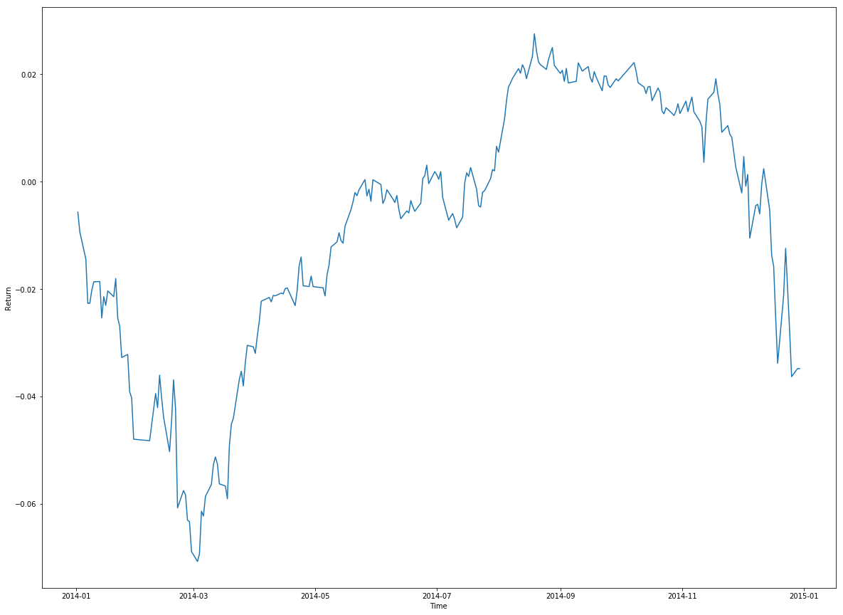
add_date_returns: [0.00015617231597244742, 0.0017472763373915876, 0.008023438642092214, 0.014377653228932943, 0.010900970332931246]

<Figure size 432x288 with 0 Axes>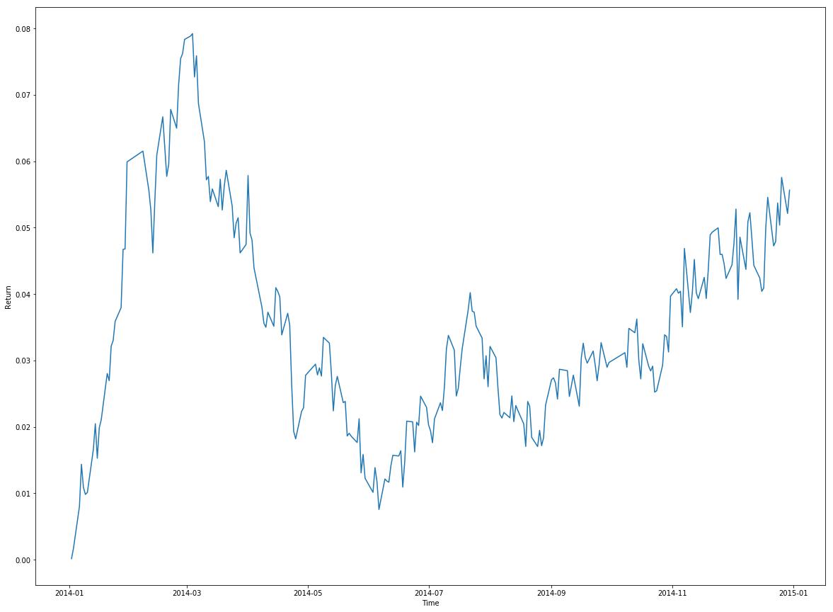
add_date_returns: [-0.005295996766264036, -0.007935137845153834, -0.0116598235794378, -0.015382549040431544, -0.01544626622160069]

<Figure size 432x288 with 0 Axes>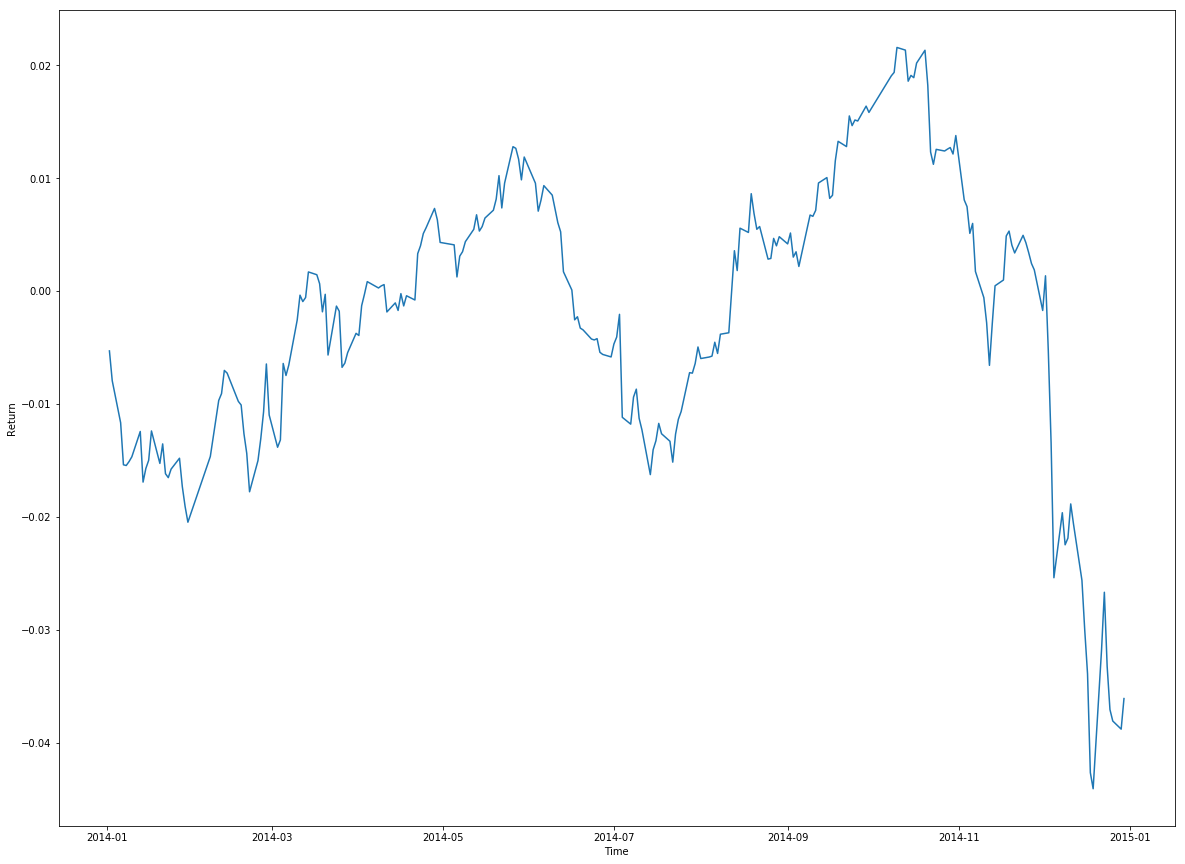
add_date_returns: [-0.004370600684310187, -0.008172362738429279, -0.014656030395962263, -0.021494493631889895, -0.020471243410280712]

<Figure size 432x288 with 0 Axes>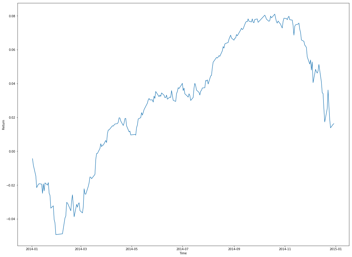
add_date_returns: [-0.0039841955418837924, -0.004729212954451003, -0.010457567287858417, -0.01908759882026042, -0.020879529057285663]

<Figure size 432x288 with 0 Axes>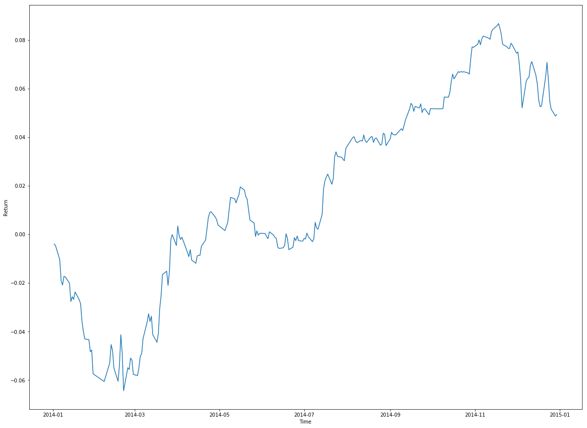
add_date_returns: [-0.005634572963722873, -0.008865408238608232, -0.012695946696617217, -0.02137327024608645, -0.023466768300461925]

<Figure size 432x288 with 0 Axes>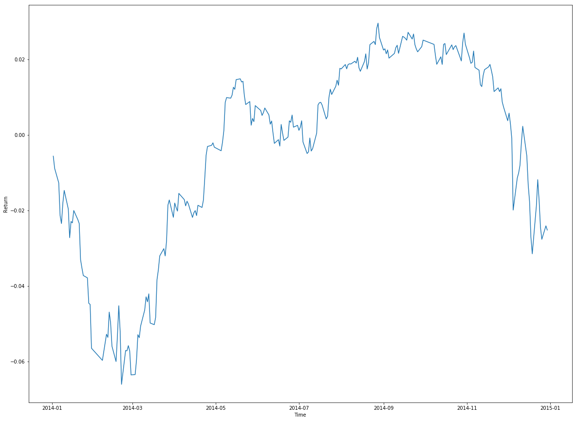
add_date_returns: [-0.0032470511593805183, -0.0056963193683139315, -0.010993355828043715, -0.018998905636241084, -0.023157852979990713]

<Figure size 432x288 with 0 Axes>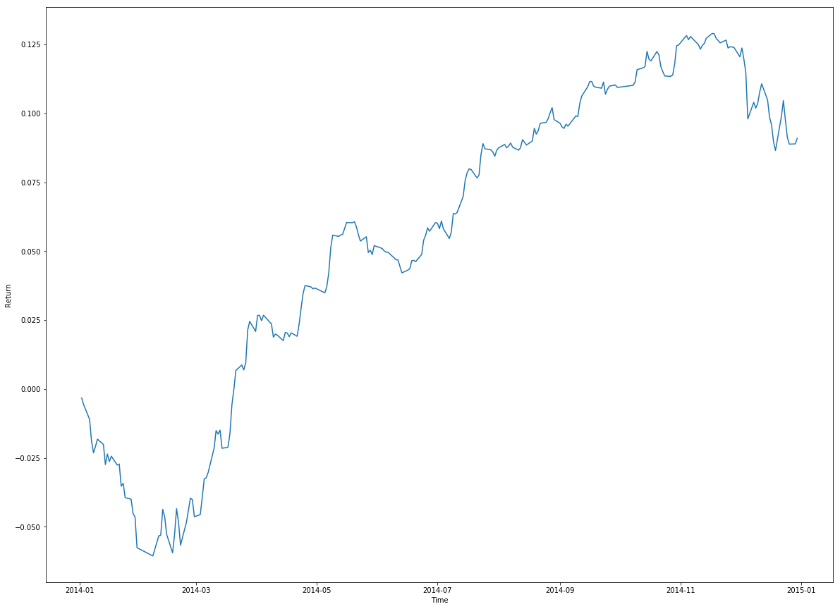
add_date_returns: [-0.004124106812945408, -0.0025554859604423018, -0.006373135502058449, -0.014053842931236186, -0.015720635786636877]

<Figure size 432x288 with 0 Axes>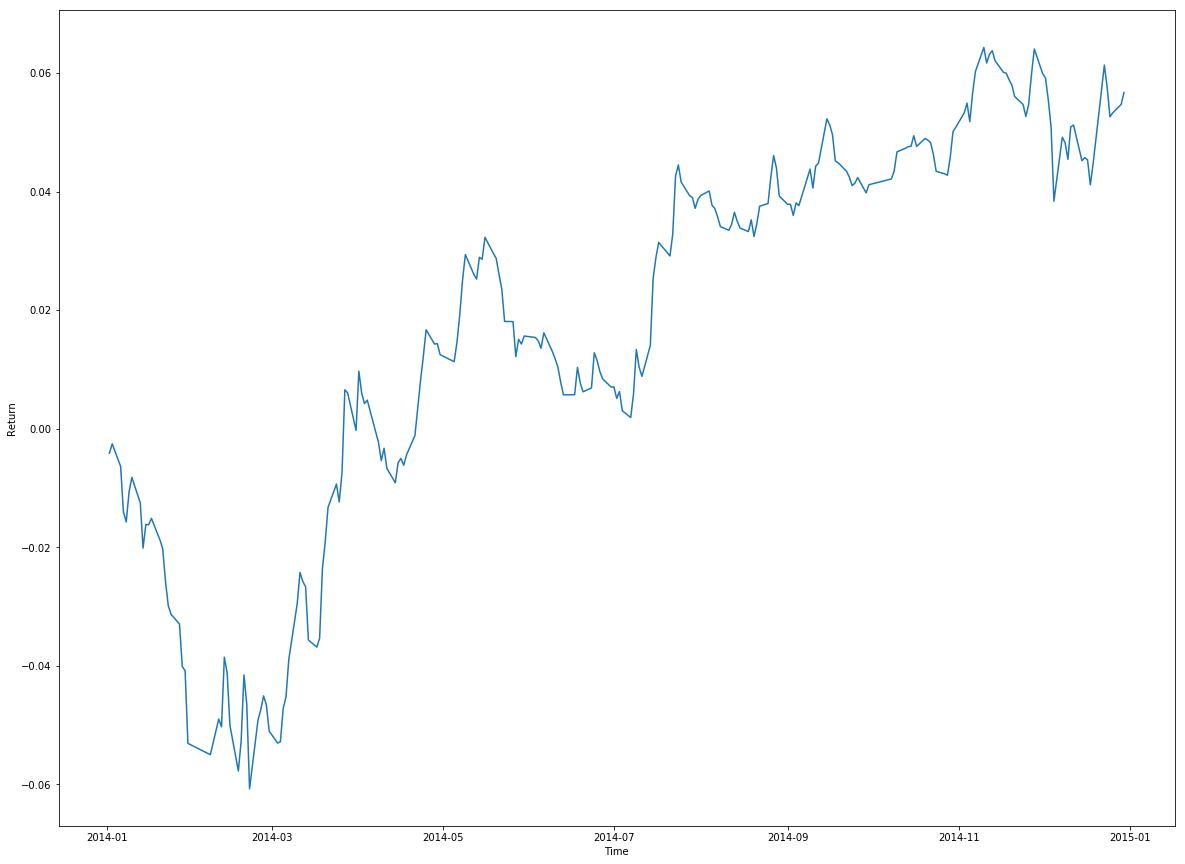
add_date_returns: [-0.0037491580077676345, -0.006012275717163283, -0.007747134202037593, -0.013074364112121576, -0.01894842836552238]

<Figure size 432x288 with 0 Axes>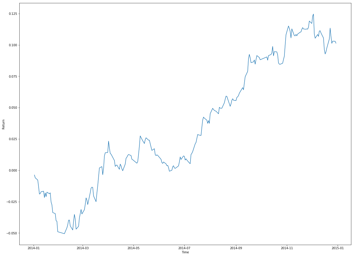
为者常成,行者常至
自由转载-非商用-非衍生-保持署名(创意共享3.0许可证)


