AI 深度学习之初始化参数

本小节大家已经看了不少文章了。可能有些同学觉得那些文章没有什么用。其实它们都是很有用的干货。我会通过3个实战编程向大家展示这些文章里面的知识是多大的强大。

第一个实战编程就是初始化参数。

训练一个神经网络模型就是要找到一组特殊的参数。这个模型配上这组参数后，就拥有了某项能力，例如可以识别猫。所以，找参数才是训练的最终目的。所以，参数的初始化非常重要。

如果参数被初始化得离理想参数很远很远，那么就需要很长很长的时间来进行梯度下降才能到达理想参数。打比方说，w的理想值是2，而你将w初始化为1000，每次梯度下降又只能使w靠近理想值1个单位，那么要进行998次梯度下降才能找到理想参数；如果将w初始化为10，那么就只需要8次。

更坏的情况是，如果参数初始化得不合理，那么有可能会导致无论怎么样训练都无法找到理想值，你的模型永远不可能被训练成功。

本次实战编程向大家展示了3种不同的初始化方法，只有初始化不同而已，其它都是一样的，但结果却有3种：一种是无法找到理想值，另外一种是很长时间才能找到理想值，最后一种却很快就找到理想值了。

# 加载系统工具库
import numpy as np
import matplotlib.pyplot as plt
import sklearn
import sklearn.datasets

# 加载自定义的工具库
from init_utils import *

# 设置好画图工具
%matplotlib inline
plt.rcParams['figure.figsize'] = (7.0, 4.0) # set default size of plots
plt.rcParams['image.interpolation'] = 'nearest'
plt.rcParams['image.cmap'] = 'gray'

# 加载我们用算法生成的假数据并把它们画出来（只画了训练数据，没有画测试数据）。
# 我们的目的就是训练一个模型，使其能够将红点和蓝点区分开。
train_X, train_Y, test_X, test_Y = load_dataset()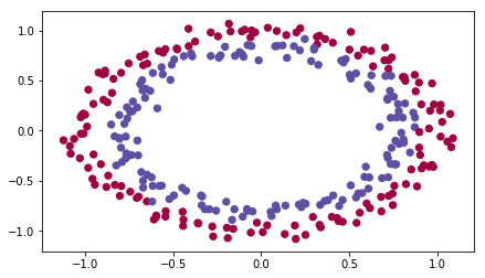

# 构建一个模型，实现细节很多都在我们自定义的工具库init_utils.py里面。因为那些细节我们之前已经学过，
# 所以为了突出重点，就把它们隐藏在工具库里面了。
# 这个模型的特点是，它可以指定3种不同的初始化方法，通过参数initialization来控制
def model(X, Y, learning_rate=0.01, num_iterations=15000, print_cost=True, initialization="he"):        
    grads = {}
    costs = [] 
    m = X.shape[1]
    layers_dims = [X.shape[0], 10, 5, 1] # 构建一个3层的神经网络

    # 3种不同的初始化方法，后面会对这3种初始化方法进行详细介绍
    if initialization == "zeros":
        parameters = initialize_parameters_zeros(layers_dims)
    elif initialization == "random":
        parameters = initialize_parameters_random(layers_dims)
    elif initialization == "he":
        parameters = initialize_parameters_he(layers_dims)

    # 梯度下降训练参数
    for i in range(0, num_iterations):
        a3, cache = forward_propagation(X, parameters)
        cost = compute_loss(a3, Y)
        grads = backward_propagation(X, Y, cache)
        parameters = update_parameters(parameters, grads, learning_rate)

        if print_cost and i % 1000 == 0:
            print("Cost after iteration {}: {}".format(i, cost))
            costs.append(cost)

    # 画出成本走向图
    plt.plot(costs)
    plt.ylabel('cost')
    plt.xlabel('iterations (per hundreds)')
    plt.title("Learning rate =" + str(learning_rate))
    plt.show()

    return parameters

# 这是我们要介绍的第一种方法。是最差的方法。也是我们学习过的第一种方法——全部初始化为0
def initialize_parameters_zeros(layers_dims):    
    parameters = {}
    L = len(layers_dims)            

    for l in range(1, L):
        parameters['W' + str(l)] = np.zeros((layers_dims[l], layers_dims[l - 1]))
        parameters['b' + str(l)] = np.zeros((layers_dims[l], 1))
    return parameters

# 单元测试
parameters = initialize_parameters_zeros([3,2,1])
print("W1 = " + str(parameters["W1"]))
print("b1 = " + str(parameters["b1"]))
print("W2 = " + str(parameters["W2"]))
print("b2 = " + str(parameters["b2"]))

W1 = [[0. 0. 0.]
 [0. 0. 0.]]
b1 = [[0.]
 [0.]]
W2 = [[0. 0.]]
b2 = [[0.]]

# 用全0初始化法进行参数训练
parameters = model(train_X, train_Y, initialization = "zeros")
print ("On the train set:")
predictions_train = predict(train_X, train_Y, parameters) # 对训练数据进行预测，并打印出准确度
print ("On the test set:")
predictions_test = predict(test_X, test_Y, parameters) # 对训测试数据进行预测，并打印出准确度

Cost after iteration 0: 0.6931471805599453
Cost after iteration 1000: 0.6931471805599453
Cost after iteration 2000: 0.6931471805599453
Cost after iteration 3000: 0.6931471805599453
Cost after iteration 4000: 0.6931471805599453
Cost after iteration 5000: 0.6931471805599453
Cost after iteration 6000: 0.6931471805599453
Cost after iteration 7000: 0.6931471805599453
Cost after iteration 8000: 0.6931471805599453
Cost after iteration 9000: 0.6931471805599453
Cost after iteration 10000: 0.6931471805599455
Cost after iteration 11000: 0.6931471805599453
Cost after iteration 12000: 0.6931471805599453
Cost after iteration 13000: 0.6931471805599453
Cost after iteration 14000: 0.6931471805599453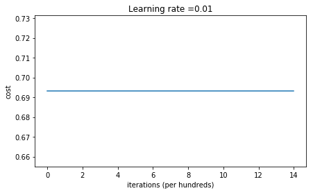

On the train set:
Accuracy: 0.5
On the test set:
Accuracy: 0.5

从上面的图表我们可以看出，成本完全没有下降，说明根本就一点都没有优化到。0.5的精确度就像赌单双一样，完全没有预测的能力。下面我们在把预测结果打印出来。可以看到，神经网络全部预测它们为0.

print("predictions_train = " + str(predictions_train))
print("predictions_test = " + str(predictions_test))

predictions_train = [[0 0 0 0 0 0 0 0 0 0 0 0 0 0 0 0 0 0 0 0 0 0 0 0 0 0 0 0 0 0 0 0 0 0 0 0
  0 0 0 0 0 0 0 0 0 0 0 0 0 0 0 0 0 0 0 0 0 0 0 0 0 0 0 0 0 0 0 0 0 0 0 0
  0 0 0 0 0 0 0 0 0 0 0 0 0 0 0 0 0 0 0 0 0 0 0 0 0 0 0 0 0 0 0 0 0 0 0 0
  0 0 0 0 0 0 0 0 0 0 0 0 0 0 0 0 0 0 0 0 0 0 0 0 0 0 0 0 0 0 0 0 0 0 0 0
  0 0 0 0 0 0 0 0 0 0 0 0 0 0 0 0 0 0 0 0 0 0 0 0 0 0 0 0 0 0 0 0 0 0 0 0
  0 0 0 0 0 0 0 0 0 0 0 0 0 0 0 0 0 0 0 0 0 0 0 0 0 0 0 0 0 0 0 0 0 0 0 0
  0 0 0 0 0 0 0 0 0 0 0 0 0 0 0 0 0 0 0 0 0 0 0 0 0 0 0 0 0 0 0 0 0 0 0 0
  0 0 0 0 0 0 0 0 0 0 0 0 0 0 0 0 0 0 0 0 0 0 0 0 0 0 0 0 0 0 0 0 0 0 0 0
  0 0 0 0 0 0 0 0 0 0 0 0]]
predictions_test = [[0 0 0 0 0 0 0 0 0 0 0 0 0 0 0 0 0 0 0 0 0 0 0 0 0 0 0 0 0 0 0 0 0 0 0 0
  0 0 0 0 0 0 0 0 0 0 0 0 0 0 0 0 0 0 0 0 0 0 0 0 0 0 0 0 0 0 0 0 0 0 0 0
  0 0 0 0 0 0 0 0 0 0 0 0 0 0 0 0 0 0 0 0 0 0 0 0 0 0 0 0]]

为什么会这样呢？这个在我们本小节的文章里面已经解释了——如果初始化参数为0，那么神经网络的每一层都只会学习到同样的东西，也就是说，一万层的神经网络和一层的单神经网络一样一样了。

为了使每一层每一个神经元都能学到不同的东西，我们需要将参数进行随机初始化。下面这个方法就是对神经网络进行参数随机初始化。

def initialize_parameters_random(layers_dims):  
    np.random.seed(3) 
    parameters = {}
    L = len(layers_dims) 

    for l in range(1, L):
        parameters['W' + str(l)] = np.random.randn(layers_dims[l], layers_dims[l - 1]) * 10
        parameters['b' + str(l)] = np.zeros((layers_dims[l], 1))
    return parameters

parameters = initialize_parameters_random([3, 2, 1])
print("W1 = " + str(parameters["W1"]))
print("b1 = " + str(parameters["b1"]))
print("W2 = " + str(parameters["W2"]))
print("b2 = " + str(parameters["b2"]))

W1 = [[ 17.88628473   4.36509851   0.96497468]
 [-18.63492703  -2.77388203  -3.54758979]]
b1 = [[0.]
 [0.]]
W2 = [[-0.82741481 -6.27000677]]
b2 = [[0.]]

parameters = model(train_X, train_Y, initialization = "random")
print("On the train set:")
predictions_train = predict(train_X, train_Y, parameters)
print("On the test set:")
predictions_test = predict(test_X, test_Y, parameters)

Cost after iteration 0: inf

C:\Users\Capta\AI blog\My\4 初始化参数\init_utils.py:145: RuntimeWarning: divide by zero encountered in log
  logprobs = np.multiply(-np.log(a3),Y) + np.multiply(-np.log(1 - a3), 1 - Y)
C:\Users\Capta\AI blog\My\4 初始化参数\init_utils.py:145: RuntimeWarning: invalid value encountered in multiply
  logprobs = np.multiply(-np.log(a3),Y) + np.multiply(-np.log(1 - a3), 1 - Y)

Cost after iteration 1000: 0.6235719528716395
Cost after iteration 2000: 0.5980821226022246
Cost after iteration 3000: 0.5637996692567824
Cost after iteration 4000: 0.5501754102867465
Cost after iteration 5000: 0.5444767640123352
Cost after iteration 6000: 0.5374657035647926
Cost after iteration 7000: 0.4775406670630984
Cost after iteration 8000: 0.39784053325714386
Cost after iteration 9000: 0.3934817369887478
Cost after iteration 10000: 0.39203280921110983
Cost after iteration 11000: 0.38927347547167324
Cost after iteration 12000: 0.3861625886188003
Cost after iteration 13000: 0.38499044850062425
Cost after iteration 14000: 0.38279756848782404

On the train set:
Accuracy: 0.83
On the test set:
Accuracy: 0.86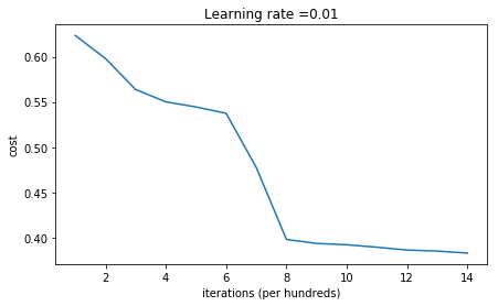

上面就是随机初始化后神经网络的表现。如果上面结果中的第一次训练后的成本是inf，请先不要在意，这个问题我们以后在讨论。

可以看出。随机初始化参数后，神经网络的表现就明显不同了。精准度提升到了0.8. 下面打印出的预测结果和图表也显示不再全部
都是零了。说明这个神经网络已经有了一些预测能力了。

print(predictions_train)
print(predictions_test)

[[1 0 1 1 0 0 1 1 1 1 1 0 1 0 0 1 0 1 1 0 0 0 1 0 1 1 1 1 1 1 0 1 1 0 0 1
  1 1 1 1 1 1 1 0 1 1 1 1 0 1 0 1 1 1 1 0 0 1 1 1 1 0 1 1 0 1 0 1 1 1 1 0
  0 0 0 0 1 0 1 0 1 1 1 0 0 1 1 1 1 1 1 0 0 1 1 1 0 1 1 0 1 0 1 1 0 1 1 0
  1 0 1 1 0 0 1 0 0 1 1 0 1 1 1 0 1 0 0 1 0 1 1 1 1 1 1 1 0 1 1 0 0 1 1 0
  0 0 1 0 1 0 1 0 1 1 1 0 0 1 1 1 1 0 1 1 0 1 0 1 1 0 1 0 1 1 1 1 0 1 1 1
  1 0 1 0 1 0 1 1 1 1 0 1 1 0 1 1 0 1 1 0 1 0 1 1 1 0 1 1 1 0 1 0 1 0 0 1
  0 1 1 0 1 1 0 1 1 0 1 1 1 0 1 1 1 1 0 1 0 0 1 1 0 1 1 1 0 0 0 1 1 0 1 1
  1 1 0 1 1 0 1 1 1 0 0 1 0 0 0 1 0 0 0 1 1 1 1 0 0 0 0 1 1 1 1 0 0 1 1 1
  1 1 1 1 0 0 0 1 1 1 1 0]]
[[1 1 1 1 0 1 0 1 1 0 1 1 1 0 0 0 0 1 0 1 0 0 1 0 1 0 1 1 1 1 1 0 0 0 0 1
  0 1 1 0 0 1 1 1 1 1 0 1 1 1 0 1 0 1 1 0 1 0 1 0 1 1 1 1 1 1 1 1 1 0 1 0
  1 1 1 1 1 0 1 0 0 1 0 0 0 1 1 0 1 1 0 0 0 1 1 0 1 1 0 0]]

plt.title("Model with large random initialization")
axes = plt.gca()
axes.set_xlim([-1.5, 1.5])
axes.set_ylim([-1.5, 1.5])
plot_decision_boundary(lambda x: predict_dec(parameters, x.T), train_X, train_Y)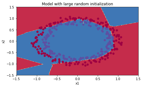

但是我们还可以继续参数的初始化方法，使神经网络更加强大。

从上面的成本图可以看出，成本开始时特别大。这是因为我们将参数初始化成了很大的值，这就会导致神经网络在前期对预测太绝对了，不是0就是1，如果预测错了，就会导致成本很大。

参数初始化得不对会导致训练效率很差，需要训练很长时间才能靠近理想值。下面的代码中，你可以将训练次数改大一些，你会看到，训练得越久，成本会越来越小，预测精准度越来越高。

参数初始化得不对，还会导致梯度消失和爆炸。

最后给大家演示一下我们文章2.1.8中提到的参数初始化方法。

def initialize_parameters_he(layers_dims):    
    np.random.seed(3)
    parameters = {}
    L = len(layers_dims) - 1

    for l in range(1, L + 1):
        parameters['W' + str(l)] = np.random.randn(layers_dims[l], layers_dims[l - 1]) * np.sqrt(2 / layers_dims[l - 1])
        parameters['b' + str(l)] = np.zeros((layers_dims[l], 1))

    return parameters

parameters = initialize_parameters_he([2, 4, 1])
print("W1 = " + str(parameters["W1"]))
print("b1 = " + str(parameters["b1"]))
print("W2 = " + str(parameters["W2"]))
print("b2 = " + str(parameters["b2"]))

W1 = [[ 1.78862847  0.43650985]
 [ 0.09649747 -1.8634927 ]
 [-0.2773882  -0.35475898]
 [-0.08274148 -0.62700068]]
b1 = [[0.]
 [0.]
 [0.]
 [0.]]
W2 = [[-0.03098412 -0.33744411 -0.92904268  0.62552248]]
b2 = [[0.]]

parameters = model(train_X, train_Y, initialization = "he")
print("On the train set:")
predictions_train = predict(train_X, train_Y, parameters)
print("On the test set:")
predictions_test = predict(test_X, test_Y, parameters)

Cost after iteration 0: 0.8830537463419761
Cost after iteration 1000: 0.6879825919728063
Cost after iteration 2000: 0.6751286264523371
Cost after iteration 3000: 0.6526117768893807
Cost after iteration 4000: 0.6082958970572938
Cost after iteration 5000: 0.5304944491717495
Cost after iteration 6000: 0.4138645817071795
Cost after iteration 7000: 0.31178034648444414
Cost after iteration 8000: 0.23696215330322565
Cost after iteration 9000: 0.18597287209206842
Cost after iteration 10000: 0.15015556280371808
Cost after iteration 11000: 0.12325079292273552
Cost after iteration 12000: 0.09917746546525931
Cost after iteration 13000: 0.08457055954024274
Cost after iteration 14000: 0.07357895962677365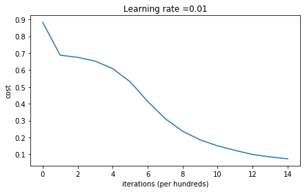

On the train set:
Accuracy: 0.9933333333333333
On the test set:
Accuracy: 0.96

plt.title("Model with He initialization")
axes = plt.gca()
axes.set_xlim([-1.5, 1.5])
axes.set_ylim([-1.5, 1.5])
plot_decision_boundary(lambda x: predict_dec(parameters, x.T), train_X, train_Y)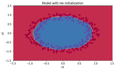

怎么样。看到上面的结果是不是很惊讶？~~ 从0.5到了0.96.神经网络其它的什么都没有变，只是改变了对参数的初始化方法。
可想而知，对参数的初始化是多么的重要。

只是运用了我们文章中的一点点知识，就使得神经网络瞬间从一个弱智变成了一个智能体。所以大家要有耐心学好每一篇文章，不要只贪图快，要真正的理解知识点。我可以向大家保证，我发布的每一篇文章，对你们将来的人工智能事业都是有帮助的。

辅助函数

init_utils.py

import numpy as np
import matplotlib.pyplot as plt
import h5py
import sklearn
import sklearn.datasets

def sigmoid(x):
    """
    Compute the sigmoid of x

    Arguments:
    x -- A scalar or numpy array of any size.

    Return:
    s -- sigmoid(x)
    """
    s = 1/(1+np.exp(-x))
    return s

def relu(x):
    """
    Compute the relu of x

    Arguments:
    x -- A scalar or numpy array of any size.

    Return:
    s -- relu(x)
    """
    s = np.maximum(0,x)

    return s

def forward_propagation(X, parameters):
    """
    Implements the forward propagation (and computes the loss) presented in Figure 2.

    Arguments:
    X -- input dataset, of shape (input size, number of examples)
    Y -- true "label" vector (containing 0 if cat, 1 if non-cat)
    parameters -- python dictionary containing your parameters "W1", "b1", "W2", "b2", "W3", "b3":
                    W1 -- weight matrix of shape ()
                    b1 -- bias vector of shape ()
                    W2 -- weight matrix of shape ()
                    b2 -- bias vector of shape ()
                    W3 -- weight matrix of shape ()
                    b3 -- bias vector of shape ()

    Returns:
    loss -- the loss function (vanilla logistic loss)
    """

    # retrieve parameters
    W1 = parameters["W1"]
    b1 = parameters["b1"]
    W2 = parameters["W2"]
    b2 = parameters["b2"]
    W3 = parameters["W3"]
    b3 = parameters["b3"]

    # LINEAR -> RELU -> LINEAR -> RELU -> LINEAR -> SIGMOID
    z1 = np.dot(W1, X) + b1
    a1 = relu(z1)
    z2 = np.dot(W2, a1) + b2
    a2 = relu(z2)
    z3 = np.dot(W3, a2) + b3
    a3 = sigmoid(z3)

    cache = (z1, a1, W1, b1, z2, a2, W2, b2, z3, a3, W3, b3)

    return a3, cache

def backward_propagation(X, Y, cache):
    """
    Implement the backward propagation presented in figure 2.

    Arguments:
    X -- input dataset, of shape (input size, number of examples)
    Y -- true "label" vector (containing 0 if cat, 1 if non-cat)
    cache -- cache output from forward_propagation()

    Returns:
    gradients -- A dictionary with the gradients with respect to each parameter, activation and pre-activation variables
    """
    m = X.shape[1]
    (z1, a1, W1, b1, z2, a2, W2, b2, z3, a3, W3, b3) = cache

    dz3 = 1./m * (a3 - Y)
    dW3 = np.dot(dz3, a2.T)
    db3 = np.sum(dz3, axis=1, keepdims = True)

    da2 = np.dot(W3.T, dz3)
    dz2 = np.multiply(da2, np.int64(a2 > 0))
    dW2 = np.dot(dz2, a1.T)
    db2 = np.sum(dz2, axis=1, keepdims = True)

    da1 = np.dot(W2.T, dz2)
    dz1 = np.multiply(da1, np.int64(a1 > 0))
    dW1 = np.dot(dz1, X.T)
    db1 = np.sum(dz1, axis=1, keepdims = True)

    gradients = {"dz3": dz3, "dW3": dW3, "db3": db3,
                 "da2": da2, "dz2": dz2, "dW2": dW2, "db2": db2,
                 "da1": da1, "dz1": dz1, "dW1": dW1, "db1": db1}

    return gradients

def update_parameters(parameters, grads, learning_rate):
    """
    Update parameters using gradient descent

    Arguments:
    parameters -- python dictionary containing your parameters 
    grads -- python dictionary containing your gradients, output of n_model_backward

    Returns:
    parameters -- python dictionary containing your updated parameters 
                  parameters['W' + str(i)] = ... 
                  parameters['b' + str(i)] = ...
    """

    L = len(parameters) // 2 # number of layers in the neural networks

    # Update rule for each parameter
    for k in range(L):
        parameters["W" + str(k+1)] = parameters["W" + str(k+1)] - learning_rate * grads["dW" + str(k+1)]
        parameters["b" + str(k+1)] = parameters["b" + str(k+1)] - learning_rate * grads["db" + str(k+1)]

    return parameters

def compute_loss(a3, Y):

    """
    Implement the loss function

    Arguments:
    a3 -- post-activation, output of forward propagation
    Y -- "true" labels vector, same shape as a3

    Returns:
    loss - value of the loss function
    """

    m = Y.shape[1]
    logprobs = np.multiply(-np.log(a3),Y) + np.multiply(-np.log(1 - a3), 1 - Y)
    loss = 1./m * np.nansum(logprobs)

    return loss

def load_cat_dataset():
    train_dataset = h5py.File('datasets/train_catvnoncat.h5', "r")
    train_set_x_orig = np.array(train_dataset["train_set_x"][:]) # your train set features
    train_set_y_orig = np.array(train_dataset["train_set_y"][:]) # your train set labels

    test_dataset = h5py.File('datasets/test_catvnoncat.h5', "r")
    test_set_x_orig = np.array(test_dataset["test_set_x"][:]) # your test set features
    test_set_y_orig = np.array(test_dataset["test_set_y"][:]) # your test set labels

    classes = np.array(test_dataset["list_classes"][:]) # the list of classes

    train_set_y = train_set_y_orig.reshape((1, train_set_y_orig.shape[0]))
    test_set_y = test_set_y_orig.reshape((1, test_set_y_orig.shape[0]))

    train_set_x_orig = train_set_x_orig.reshape(train_set_x_orig.shape[0], -1).T
    test_set_x_orig = test_set_x_orig.reshape(test_set_x_orig.shape[0], -1).T

    train_set_x = train_set_x_orig/255
    test_set_x = test_set_x_orig/255

    return train_set_x, train_set_y, test_set_x, test_set_y, classes

def predict(X, y, parameters):
    """
    This function is used to predict the results of a  n-layer neural network.

    Arguments:
    X -- data set of examples you would like to label
    parameters -- parameters of the trained model

    Returns:
    p -- predictions for the given dataset X
    """

    m = X.shape[1]
    p = np.zeros((1,m), dtype = np.int)

    # Forward propagation
    a3, caches = forward_propagation(X, parameters)

    # convert probas to 0/1 predictions
    for i in range(0, a3.shape[1]):
        if a3[0,i] > 0.5:
            p[0,i] = 1
        else:
            p[0,i] = 0

    # print results
    print("Accuracy: "  + str(np.mean((p[0,:] == y[0,:]))))

    return p

def plot_decision_boundary(model, X, y):
    # Set min and max values and give it some padding
    x_min, x_max = X[0, :].min() - 1, X[0, :].max() + 1
    y_min, y_max = X[1, :].min() - 1, X[1, :].max() + 1
    h = 0.01
    # Generate a grid of points with distance h between them
    xx, yy = np.meshgrid(np.arange(x_min, x_max, h), np.arange(y_min, y_max, h))
    # Predict the function value for the whole grid
    Z = model(np.c_[xx.ravel(), yy.ravel()])
    Z = Z.reshape(xx.shape)
    # Plot the contour and training examples
    plt.contourf(xx, yy, Z, cmap=plt.cm.Spectral)
    plt.ylabel('x2')
    plt.xlabel('x1')
    plt.scatter(X[0, :], X[1, :], c=y.ravel(), cmap=plt.cm.Spectral)
    plt.show()

def predict_dec(parameters, X):
    """
    Used for plotting decision boundary.

    Arguments:
    parameters -- python dictionary containing your parameters 
    X -- input data of size (m, K)

    Returns
    predictions -- vector of predictions of our model (red: 0 / blue: 1)
    """

    # Predict using forward propagation and a classification threshold of 0.5
    a3, cache = forward_propagation(X, parameters)
    predictions = (a3>0.5)
    return predictions

def load_dataset():
    np.random.seed(1)
    train_X, train_Y = sklearn.datasets.make_circles(n_samples=300, noise=.05)
    np.random.seed(2)
    test_X, test_Y = sklearn.datasets.make_circles(n_samples=100, noise=.05)
    # Visualize the data
    plt.scatter(train_X[:, 0], train_X[:, 1], c=train_Y, s=40, cmap=plt.cm.Spectral);
    train_X = train_X.T
    train_Y = train_Y.reshape((1, train_Y.shape[0]))
    test_X = test_X.T
    test_Y = test_Y.reshape((1, test_Y.shape[0]))
    return train_X, train_Y, test_X, test_Y

为者常成，行者常至