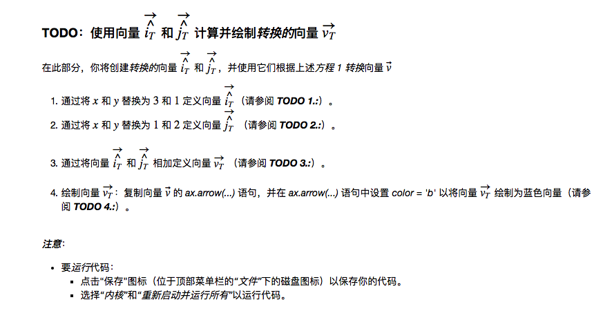
Python:线性代数-线性映射实战 Lab (五十二)

说明

对于第一道 Lab 练习可视化矩阵乘法，你将使用一个简单的 Python 示例可视化矩阵乘法的流程。第一道练习介绍了矩阵乘法流程。

对于第二道练习矩阵乘法 Lab，你将在 Python 中使用矩阵乘法解决一个更复杂的问题。第二道练习演示了如何使用矩阵乘法解决更复杂的问题，例如将在 AI 中遇到的神经网络问题。

可视化矩阵乘法

绘制分解为基向量 ?̂ ⃗ 和 ?̂ ⃗ 的向量 ?⃗

 Import NumPy and Matplotlib
%matplotlib inline
import numpy as np
import matplotlib.pyplot as plt

# Define vector v 
v = np.array([-1,2])

# Define basis vector i_hat as unit vector
i_hat = np.array([1,0])

# Define basis vector j_hat as unit vector
j_hat = np.array([0,1])

# Define v_ihat - as v[0](x) multiplied by basis vector ihat
v_ihat = v[0] * i_hat

# Define v_jhat_t - as v[1](y) multiplied by basis vector jhat
v_jhat = v[1] * j_hat

# Plot that graphically shows vector v (color='b') - whose position can be  
# decomposed into v_ihat and v_jhat 

# Creates axes of plot referenced 'ax'
ax = plt.axes()

# Plots red dot at origin (0,0)
ax.plot(0,0,'or')

# Plots vector v_ihat as dotted green arrow starting at origin 0,0
ax.arrow(0, 0, *v_ihat, color='g', linestyle='dotted', linewidth=2.5, head_width=0.30,
         head_length=0.35)

# Plots vector v_jhat as dotted red arrow starting at origin defined by v_ihat
ax.arrow(v_ihat[0], v_ihat[1], *v_jhat, color='r', linestyle='dotted', linewidth=2.5,
         head_width=0.30, head_length=0.35)

# Plots vector v as blue arrow starting at origin 0,0
ax.arrow(0, 0, *v, color='b', linewidth=2.5, head_width=0.30, head_length=0.35)

# Sets limit for plot for x-axis
plt.xlim(-4, 2)

# Set major ticks for x-axis
major_xticks = np.arange(-4, 2)
ax.set_xticks(major_xticks)

# Sets limit for plot for y-axis
plt.ylim(-2, 4)

# Set major ticks for y-axis
major_yticks = np.arange(-2, 4)
ax.set_yticks(major_yticks)

# Creates gridlines for only major tick marks
plt.grid(b=True, which='major')

# Displays final plot
plt.show()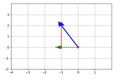

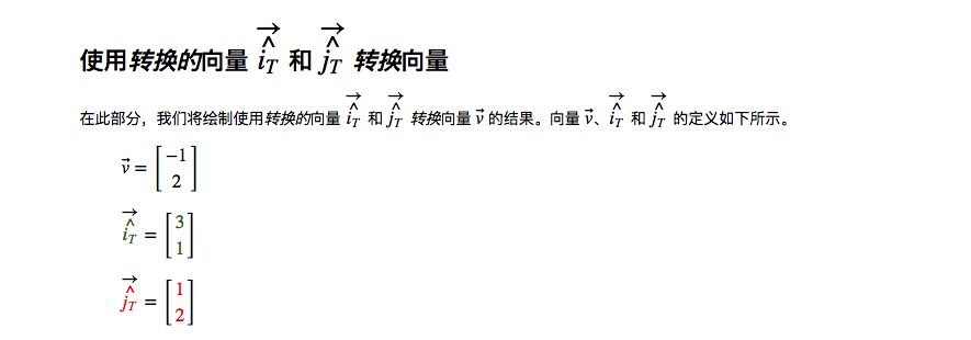
v = np.array([-1, 2])

# TODO 1.: Define vector i_hat as transformed vector i_hat(ihat_t)
# where x=3 and y=1 instead of x=1 and y=0
ihat_t = np.array([3, 1])

# TODO 2.: Define vector j_hat as transformed vector j_hat(jhat_t)
# where x=1 and y=2 instead of x=0 and y=1
jhat_t = np.array([1, 2])

# Define v_ihat_t - as v[0](x) multiplied by transformed vector ihat
v_ihat_t = v[0] * ihat_t

# Define v_jhat_t - as v[1](y) multiplied by transformed vector jhat
v_jhat_t = v[1] * jhat_t

# TODO 3.: Define transformed vector v (v_t) as 
# vector v_ihat_t added to vector v_jhat_t
v_t = v_ihat_t + v_jhat_t

# Plot that graphically shows vector v (color='skyblue') can be transformed 
# into transformed vector v (v_trfm - color='b') by adding v[0]*transformed 
# vector ihat to v[0]*transformed vector jhat

# Creates axes of plot referenced 'ax'
ax = plt.axes()

# Plots red dot at origin (0,0)
ax.plot(0,0,'or')

# Plots vector v_ihat_t as dotted green arrow starting at origin 0,0
ax.arrow(0, 0, *v_ihat_t, color='g', linestyle='dotted', linewidth=2.5, head_width=0.30,
         head_length=0.35)

# Plots vector v_jhat_t as dotted red arrow starting at origin defined by v_ihat
ax.arrow(v_ihat_t[0], v_ihat_t[1], *v_jhat_t, color='r', linestyle='dotted', linewidth=2.5,
         head_width=0.30, head_length=0.35)

# Plots vector v as blue arrow starting at origin 0,0
ax.arrow(0, 0, *v, color='skyblue', linewidth=2.5, head_width=0.30, head_length=0.35)

# TODO 4.: Plot transformed vector v (v_t) a blue colored vector(color='b') using 
# vector v's ax.arrow() statement above as template for the plot 
ax.arrow(0, 0, *v_t, color='b', linewidth=2.5, head_width=0.30, head_length=0.35)

# Sets limit for plot for x-axis
plt.xlim(-4, 2)

# Set major ticks for x-axis
major_xticks = np.arange(-4, 2)
ax.set_xticks(major_xticks)

# Sets limit for plot for y-axis
plt.ylim(-2, 4)

# Set major ticks for y-axis
major_yticks = np.arange(-2, 4)
ax.set_yticks(major_yticks)

# Creates gridlines for only major tick marks
plt.grid(b=True, which='major')

# Displays final plot
plt.show()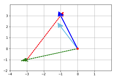

矩阵乘法

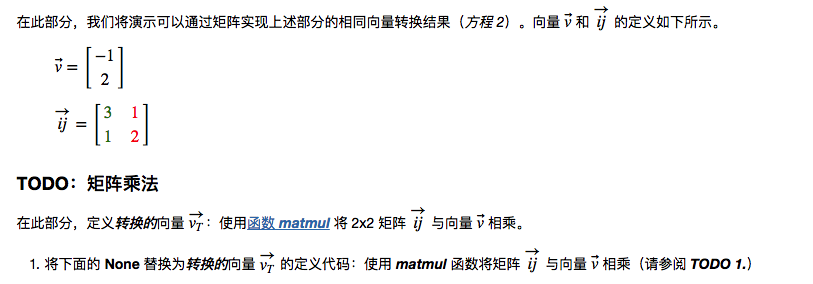
# Define vector v 
v = np.array([-1,2])

# Define 2x2 matrix ij
ij = np.array([[3, 1],[1, 2]])

# TODO 1.: Demonstrate getting v_trfm by matrix multiplication
# by using matmul function to multiply 2x2 matrix ij by vector v
# to compute the transformed vector v (v_t) 
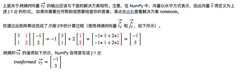
v_t = np.matmul(ij, v)

# Prints vectors v, ij, and v_t
print("\nMatrix ij:", ij, "\nVector v:", v, "\nTransformed Vector v_t:", v_t, sep="\n")

Matrix ij:
[[3 1]
[1 2]]

Vector v:
[-1 2]

Transformed Vector v_t:
[-1 3]

矩阵乘法的解决方案

为者常成，行者常至