
AI For Trading: Project1-Trading with Momentum (13)
Project Description
Trading with Momentum Project
In this project, you will learn to implement a trading strategy on your own, and test to see if it has the potential to be profitable. You will be supplied with a universe of stocks and time range. You will also be provided with a textual description of how to generate a trading signal based on a momentum indicator. You will then compute the signal for the time range given and apply it to the dataset to produce projected returns. Finally, you will perform a statistical test on the mean of the returns to conclude if there is alpha in the signal. For the dataset, we'll be using the end of day from Quotemedia.
在这个项目中,您将学习自己实施交易策略,并测试它是否有可能盈利。您将获得一系列股票和时间范围。您还将获得有关如何根据动量指标生成交易信号的文字说明。然后,您将计算给定时间范围的信号,并将其应用于数据集以生成预计回报。最后,如果信号中存在alpha,您将对返回的平均值进行统计测试。对于数据集,我们将使用Quotemedia的结束日期。
project
Project 1: Trading with Momentum
Instructions
Each problem consists of a function to implement and instructions on how to implement the function. The parts of the function that need to be implemented are marked with a # TODO comment. After implementing the function, run the cell to test it against the unit tests we've provided. For each problem, we provide one or more unit tests from our project_tests package. These unit tests won't tell you if your answer is correct, but will warn you of any major errors. Your code will be checked for the correct solution when you submit it to Udacity.
Packages
When you implement the functions, you'll only need to you use the packages you've used in the classroom, like Pandas and Numpy. These packages will be imported for you. We recommend you don't add any import statements, otherwise the grader might not be able to run your code.
The other packages that we're importing are helper, project_helper, and project_tests. These are custom packages built to help you solve the problems. The helper and project_helper module contains utility functions and graph functions. The project_tests contains the unit tests for all the problems.
Install Packages
import sys
!{sys.executable} -m pip install -r requirements.txt
Requirement already satisfied: colour==0.1.5 in /opt/conda/lib/python3.6/site-packages (from -r requirements.txt (line 1))
Collecting cvxpy==1.0.3 (from -r requirements.txt (line 2))
Downloading https://files.pythonhosted.org/packages/a1/59/2613468ffbbe3a818934d06b81b9f4877fe054afbf4f99d2f43f398a0b34/cvxpy-1.0.3.tar.gz (880kB)
[K 100% |████████████████████████████████| 880kB 520kB/s eta 0:00:01
[?25hRequirement already satisfied: cycler==0.10.0 in /opt/conda/lib/python3.6/site-packages/cycler-0.10.0-py3.6.egg (from -r requirements.txt (line 3))
Collecting numpy==1.13.3 (from -r requirements.txt (line 4))
Downloading https://files.pythonhosted.org/packages/57/a7/e3e6bd9d595125e1abbe162e323fd2d06f6f6683185294b79cd2cdb190d5/numpy-1.13.3-cp36-cp36m-manylinux1_x86_64.whl (17.0MB)
You should consider upgrading via the 'pip install --upgrade pip' command.Load Packages
import pandas as pd
import numpy as np
import helper
import project_helper
import project_tests
Market Data
Load Data
The data we use for most of the projects is end of day data. This contains data for many stocks, but we'll be looking at stocks in the S&P 500. We also made things a little easier to run by narrowing down our range of time period instead of using all of the data.
df = pd.read_csv('../../data/project_1/eod-quotemedia.csv', parse_dates=['date'], index_col=False)

close = df.reset_index().pivot(index='date', columns='ticker', values='adj_close')
#print(close)
print('Loaded Data')
Loaded DataView Data
Run the cell below to see what the data looks like for close.
project_helper.print_dataframe(close)
Stock Example
Let's see what a single stock looks like from the closing prices. For this example and future display examples in this project, we'll use Apple's stock (AAPL). If we tried to graph all the stocks, it would be too much information.
apple_ticker = 'AAPL'
project_helper.plot_stock(close[apple_ticker], '{} Stock'.format(apple_ticker))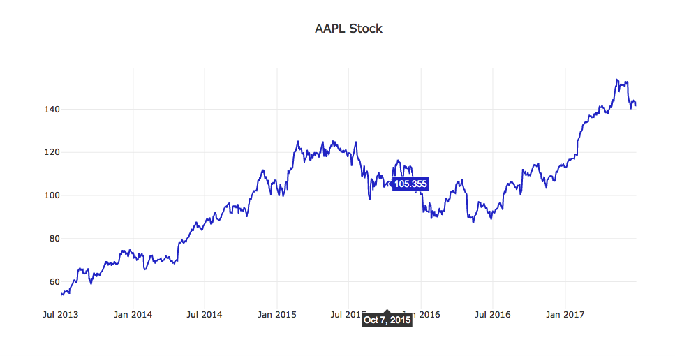
Resample Adjusted Prices
The trading signal you'll develop in this project does not need to be based on daily prices, for instance, you can use month-end prices to perform trading once a month. To do this, you must first resample the daily adjusted closing prices into monthly buckets, and select the last observation of each month.
Implement the resample_prices to resample close_prices at the sampling frequency of freq.
def resample_prices(close_prices, freq='M'):
    """
    Resample close prices for each ticker at specified frequency.

    Parameters
    ----------
    close_prices : DataFrame
        Close prices for each ticker and date
    freq : str
        What frequency to sample at
        For valid freq choices, see http://pandas.pydata.org/pandas-docs/stable/timeseries.html#offset-aliases

    Returns
    -------
    prices_resampled : DataFrame
        Resampled prices for each ticker and date
    """
    # TODO: Implement Function
    res = close_prices.groupby(pd.Grouper(freq=freq)).last()

    # print(res)

    return res

project_tests.test_resample_prices(resample_prices)
Tests PassedView Data
Let's apply this function to close and view the results.
monthly_close = resample_prices(close)
project_helper.plot_resampled_prices(
    monthly_close.loc[:, apple_ticker],
    close.loc[:, apple_ticker],
    '{} Stock - Close Vs Monthly Close'.format(apple_ticker))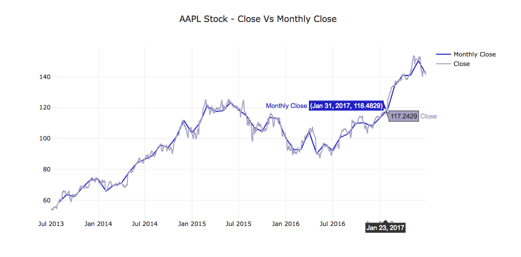
Compute Log Returns
Compute log returns ($R_t$) from prices ($P_t$) as your primary momentum indicator:
$$R_t = log_e(P_t) - loge(P{t-1})$$
Implement the compute_log_returns function below, such that it accepts a dataframe (like one returned by resample_prices), and produces a similar dataframe of log returns. Use Numpy's log function to help you calculate the log returns.
def compute_log_returns(prices):
    """
    Compute log returns for each ticker.

    Parameters
    ----------
    prices : DataFrame
        Prices for each ticker and date

    Returns
    -------
    log_returns : DataFrame
        Log returns for each ticker and date
    """
    # TODO: Implement Function

    return np.log(prices) - np.log(prices.shift(1))

project_tests.test_compute_log_returns(compute_log_returns)
Tests PassedView Data
Using the same data returned from resample_prices, we'll generate the log returns.
monthly_close_returns = compute_log_returns(monthly_close)
project_helper.plot_returns(
    monthly_close_returns.loc[:, apple_ticker],
    'Log Returns of {} Stock (Monthly)'.format(apple_ticker))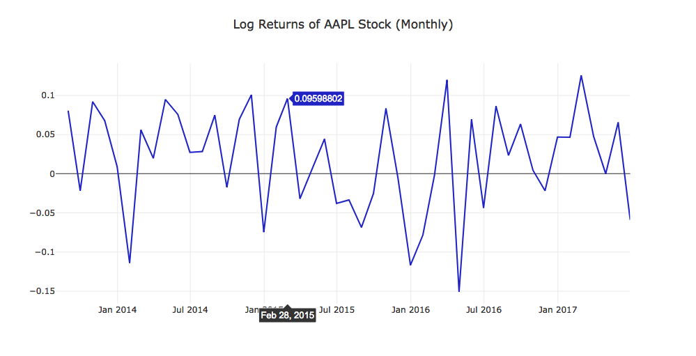
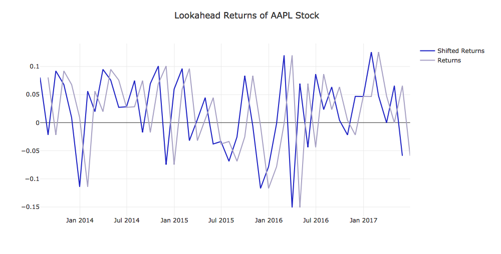
Shift Returns
Implement the shift_returns function to shift the log returns to the previous or future returns in the time series. For example, the parameter shift_n is 2 and returns is the following:
                           Returns
               A         B         C         D
2013-07-08     0.015     0.082     0.096     0.020     ...
2013-07-09     0.037     0.095     0.027     0.063     ...
2013-07-10     0.094     0.001     0.093     0.019     ...
2013-07-11     0.092     0.057     0.069     0.087     ...
...            ...       ...       ...       ...
the output of the shift_returns function would be:
                        Shift Returns
               A         B         C         D
2013-07-08     NaN       NaN       NaN       NaN       ...
2013-07-09     NaN       NaN       NaN       NaN       ...
2013-07-10     0.015     0.082     0.096     0.020     ...
2013-07-11     0.037     0.095     0.027     0.063     ...
...            ...       ...       ...       ...
Using the same returns data as above, the shift_returns function should generate the following with shift_n as -2:
                        Shift Returns
               A         B         C         D
2013-07-08     0.094     0.001     0.093     0.019     ...
2013-07-09     0.092     0.057     0.069     0.087     ...
...            ...       ...       ...       ...       ...
...            ...       ...       ...       ...       ...
...            NaN       NaN       NaN       NaN       ...
...            NaN       NaN       NaN       NaN       ...
Note: The "..." represents data points we're not showing.
def shift_returns(returns, shift_n):
    """
    Generate shifted returns

    Parameters
    ----------
    returns : DataFrame
        Returns for each ticker and date
    shift_n : int
        Number of periods to move, can be positive or negative

    Returns
    -------
    shifted_returns : DataFrame
        Shifted returns for each ticker and date
    """
    # TODO: Implement Function
    # print res
    res = returns.shift(shift_n)
    # print(res)

    return res

project_tests.test_shift_returns(shift_returns)
Tests PassedView Data
Let's get the previous month's and next month's returns.
prev_returns = shift_returns(monthly_close_returns, 1)
lookahead_returns = shift_returns(monthly_close_returns, -1)

project_helper.plot_shifted_returns(
    prev_returns.loc[:, apple_ticker],
    monthly_close_returns.loc[:, apple_ticker],
    'Previous Returns of {} Stock'.format(apple_ticker))
project_helper.plot_shifted_returns(
    lookahead_returns.loc[:, apple_ticker],
    monthly_close_returns.loc[:, apple_ticker],
    'Lookahead Returns of {} Stock'.format(apple_ticker))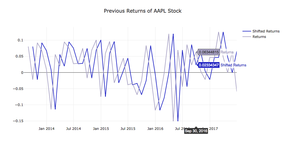
Generate Trading Signal
A trading signal is a sequence of trading actions, or results that can be used to take trading actions. A common form is to produce a "long" and "short" portfolio of stocks on each date (e.g. end of each month, or whatever frequency you desire to trade at). This signal can be interpreted as rebalancing your portfolio on each of those dates, entering long ("buy") and short ("sell") positions as indicated.
Here's a strategy that we will try:
For each month-end observation period, rank the stocks by previous returns, from the highest to the lowest. Select the top performing stocks for the long portfolio, and the bottom performing stocks for the short portfolio.
Implement the get_top_n function to get the top performing stock for each month. Get the top performing stocks from prev_returns by assigning them a value of 1. For all other stocks, give them a value of 0. For example, using the following prev_returns:
                                     Previous Returns
               A         B         C         D         E         F         G
2013-07-08     0.015     0.082     0.096     0.020     0.075     0.043     0.074
2013-07-09     0.037     0.095     0.027     0.063     0.024     0.086     0.025
...            ...       ...       ...       ...       ...       ...       ...
The function get_top_n with top_n set to 3 should return the following:
                                     Previous Returns
               A         B         C         D         E         F         G
2013-07-08     0         1         1         0         1         0         0
2013-07-09     0         1         0         1         0         1         0
...            ...       ...       ...       ...       ...       ...       ...
Note: You may have to use Panda's DataFrame.iterrows with Series.nlargest in order to implement the function. This is one of those cases where creating a vecorization solution is too difficult.
def get_top_n(prev_returns, top_n):
    """
    Select the top performing stocks

    Parameters
    ----------
    prev_returns : DataFrame
        Previous shifted returns for each ticker and date
    top_n : int
        The number of top performing stocks to get

    Returns
    -------
    top_stocks : DataFrame
        Top stocks for each ticker and date marked with a 1
    """
    # TODO: Implement Function
    # use lambda to compute
    top_stocks = prev_returns.apply(lambda x: x.nlargest(top_n), axis=1)
    # print res
    # print(top_stocks) replace na to 0 or 1
    top_stocks = top_stocks.applymap(lambda x: 0 if pd.isna(x) else 1)
    top_stocks = top_stocks.astype(np.int64)
    # print(top_stocks)

    return top_stocks

project_tests.test_get_top_n(get_top_n)
Tests PassedView Data
We want to get the best performing and worst performing stocks. To get the best performing stocks, we'll use the get_top_n function. To get the worst performing stocks, we'll also use the get_top_n function. However, we pass in -1*prev_returns instead of just prev_returns. Multiplying by negative one will flip all the positive returns to negative and negative returns to positive. Thus, it will return the worst performing stocks.
top_bottom_n = 50
df_long = get_top_n(prev_returns, top_bottom_n)
df_short = get_top_n(-1*prev_returns, top_bottom_n)
project_helper.print_top(df_long, 'Longed Stocks')
project_helper.print_top(df_short, 'Shorted Stocks')
10 Most Longed Stocks:
INCY, AMD, AVGO, NFX, NFLX, SWKS, ILMN, NVDA, UAL, MU
10 Most Shorted Stocks:
RRC, CHK, FCX, MRO, FTI, DVN, GPS, WYNN, SPLS, MATProjected Returns
It's now time to check if your trading signal has the potential to become profitable!
We'll start by computing the net returns this portfolio would return. For simplicity, we'll assume every stock gets an equal dollar amount of investment. This makes it easier to compute a portfolio's returns as the simple arithmetic average of the individual stock returns.
Implement the portfolio_returns function to compute the expected portfolio returns. Using df_long to indicate which stocks to long and df_short to indicate which stocks to short, calculate the returns using lookahead_returns. To help with calculation, we've provided you with n_stocks as the number of stocks we're investing in a single period.
def portfolio_returns(df_long, df_short, lookahead_returns, n_stocks):
    """
    Compute expected returns for the portfolio, assuming equal investment in each long/short stock.

    Parameters
    ----------
    df_long : DataFrame
        Top stocks for each ticker and date marked with a 1
    df_short : DataFrame
        Bottom stocks for each ticker and date marked with a 1
    lookahead_returns : DataFrame
        Lookahead returns for each ticker and date
    n_stocks: int
        The number number of stocks chosen for each month

    Returns
    -------
    portfolio_returns : DataFrame
        Expected portfolio returns for each ticker and date
    """
    # TODO: Implement Function
    # print("lookahead_returns:")
    # print(lookahead_returns)
    # print()

    # print("df_long:")
    # print(df_long)
    # print()

    #print("df_short:")
    #print(df_short)
    #print()

    #print("n_stocks:")
    #print(n_stocks)
    #print()

    res = (lookahead_returns*(df_long - df_short)) / n_stocks

    # print res
    # print("res:")
    # print(res)

    return res

project_tests.test_portfolio_returns(portfolio_returns)
Tests PassedView Data
Time to see how the portfolio did.
expected_portfolio_returns = portfolio_returns(df_long, df_short, lookahead_returns, 2*top_bottom_n)
project_helper.plot_returns(expected_portfolio_returns.T.sum(), 'Portfolio Returns')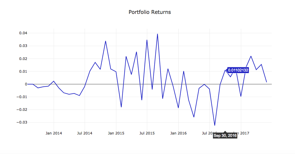
Statistical Tests
Annualized Rate of Return
expected_portfolio_returns_by_date = expected_portfolio_returns.T.sum().dropna()
portfolio_ret_mean = expected_portfolio_returns_by_date.mean()
portfolio_ret_ste = expected_portfolio_returns_by_date.sem()
portfolio_ret_annual_rate = (np.exp(portfolio_ret_mean * 12) - 1) * 100

print("""
Mean:                       {:.6f}
Standard Error:             {:.6f}
Annualized Rate of Return:  {:.2f}%
""".format(portfolio_ret_mean, portfolio_ret_ste, portfolio_ret_annual_rate))
Mean: 0.003076
Standard Error: 0.002180
Annualized Rate of Return: 3.76%The annualized rate of return allows you to compare the rate of return from this strategy to other quoted rates of return, which are usually quoted on an annual basis.
T-Test
Our null hypothesis ($H_0$) is that the actual mean return from the signal is zero. We'll perform a one-sample, one-sided t-test on the observed mean return, to see if we can reject $H_0$.
We'll need to first compute the t-statistic, and then find its corresponding p-value. The p-value will indicate the probability of observing a t-statistic equally or more extreme than the one we observed if the null hypothesis were true. A small p-value means that the chance of observing the t-statistic we observed under the null hypothesis is small, and thus casts doubt on the null hypothesis. It's good practice to set a desired level of significance or alpha ($\alpha$) before computing the p-value, and then reject the null hypothesis if $p < \alpha$.
For this project, we'll use $\alpha = 0.05$, since it's a common value to use.
Implement the analyze_alpha function to perform a t-test on the sample of portfolio returns. We've imported the scipy.stats module for you to perform the t-test.
Note: scipy.stats.ttest_1samp performs a two-sided test, so divide the p-value by 2 to get 1-sided p-value
from scipy import stats

def analyze_alpha(expected_portfolio_returns_by_date):
    """
    Perform a t-test with the null hypothesis being that the expected mean return is zero.

    Parameters
    ----------
    expected_portfolio_returns_by_date : Pandas Series
        Expected portfolio returns for each date

    Returns
    -------
    t_value
        T-statistic from t-test
    p_value
        Corresponding p-value
    """
    # TODO: Implement Function
    t_test_results = stats.ttest_1samp(expected_portfolio_returns_by_date, 0)
    t_value = t_test_results[0]
    p_value = t_test_results[1] / 2

    return t_value, p_value

project_tests.test_analyze_alpha(analyze_alpha)
Tests PassedView Data
Let's see what values we get with our portfolio. After you run this, make sure to answer the question below.
t_value, p_value = analyze_alpha(expected_portfolio_returns_by_date)
print("""
Alpha analysis:
 t-value:        {:.3f}
 p-value:        {:.6f}
""".format(t_value, p_value))
Alpha analysis:
t-value: 1.411
p-value: 0.082517Question: What p-value did you observe? And what does that indicate about your signal?
#TODO: Put Answer In this Cell
My p-value is 0.082517, and this is greater than our α of 0.05.
Submission
Now that you're done with the project, it's time to submit it. Click the submit button in the bottom right. One of our reviewers will give you feedback on your project with a pass or not passed grade. You can continue to the next section while you wait for feedback.
为者常成,行者常至
自由转载-非商用-非衍生-保持署名(创意共享3.0许可证)


